Intersection over Union (IoU)

When training an object detection model, you have surely stumbled across the Intersection over Union, in short IoU. In this short post, I will explain what it is and how to implement it in native Python. Furthermore, I will describe the implementation in Tensorflow using vector operations, so that it can be efficiently used for measuring the accuracy of an object detection model.

What is the IoU?

The Intersection over Union (IoU or Jaccard index) is a metric for measuring the accuracy of an object detection model. Imagine you have two bounding boxes, one predicted bounding box and one ground truth bounding box, and you want some indication of how good the prediction is. That’s where the Intersection over Union comes into place.

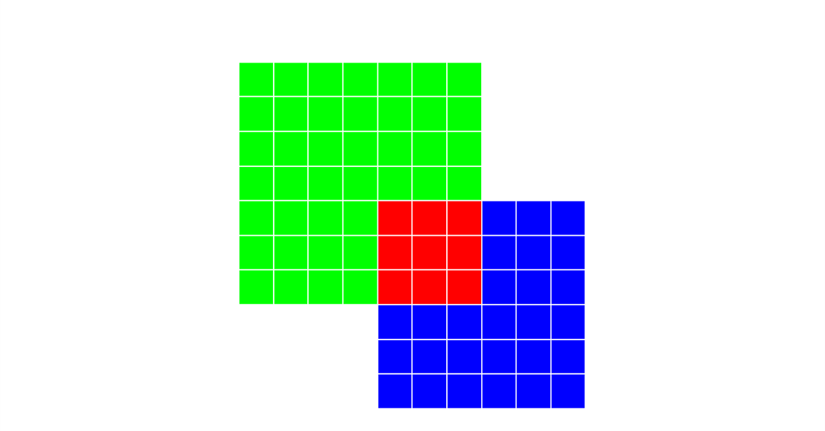
Shortly described: The Intersection over Union measures the overlap between the two bounding boxes. A resulting value of 1 indicates perfect prediction, while lower values suggest a poor prediction accuracy.

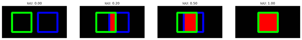
The figure below shows two bounding boxes (green and blue). In the left-most one there is no overlap, hence, the Intersection over Union equals 0 (bad prediction). But as the overlap increases (moving to the right), also the IoU increases, until the IoU is 1 for two bounding boxes that are congruent (perfect prediction).

Intuitive Example

For a more intuitive understanding let’s have a look at an example. In the picture below two rectangles A (green) and B (blue) are displayed. Rectangle A has a width and height of 7, while B has a width and height of 6 (both in pixels).

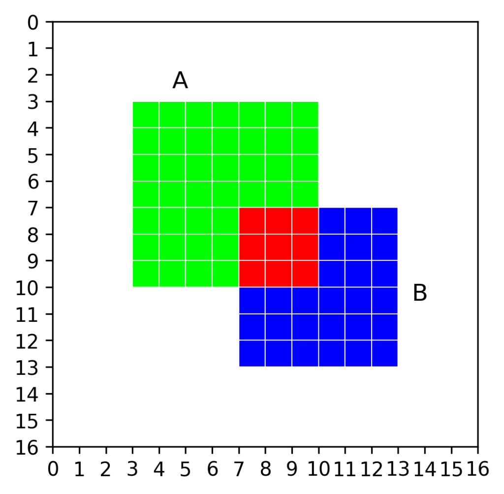
The IoU can now be described as the area of overlap divided by the area of the union. So: .

For our concrete example the intersecting area (red) is

   

The area of A (green) is

   

and the area of B (blue) is

   

The union of A and B can be computed as

   

   

Now we can compute the Intersection over Union by dividing the intersection through the union of A and B, which yields an IoU of

   

Naive Implementation

Now let’s put everything what we’ve done so far in a function that get’s two bounding boxes as input and returns the Intersection over Union. The bounding boxes have the form (𝑥, 𝑦, 𝑤, ℎ), with 𝑥 and 𝑦 being the coordinates of the top-left corner, and 𝑤 and ℎ being the width and height of the box, respectively.

def computeIoU(bbox1, bbox2):
    (x1, y1, w1, h1) = bbox1
    (x2, y2, w2, h2) = bbox2
    
    # Firstly, we calculate the areas of each box
    # by multiplying its height with its width.
    area1 = w1 * h1
    area2 = w2 * h2
    
    # Secondly, we determine the intersection
    # rectangle. For that, we try to find the
    # corner points (top-left and bottom-right)
    # of the intersection rectangle.
    inter_x1 = max(x1, x2)
    inter_y1 = max(y1, y2)
    inter_x2 = min(x1 + w1, x2 + w2)
    inter_y2 = min(y1 + h1, y2 + h2)
    
    # From the two corner points we compute the
    # width and height.
    inter_w = max(0, inter_x2 - inter_x1) 
    inter_h = max(0, inter_y2 - inter_y1)
        
    # If the width or height are equal or less than zero
    # the boxes do not overlap. Hence, the IoU equals 0.
    if inter_w <= 0 or inter_h <= 0:
        return 0.0
    # Otherwise, return the IoU (intersection area divided
    # by the union)
    else:
        inter_area = inter_w * inter_h
        return inter_area / float(area1 + area2 - inter_area)

Let’s compute the IoU for a few examples:

# example from above
iou = computeIoU((3, 3, 7, 7), (7, 7, 6, 6))
print("IoU Example: %.4f" % iou)

# congruent bounding boxes
iou = computeIoU((3, 4, 10, 10), (3, 4, 10, 10))
print("IoU Congruent: %.4f" % iou)

# non overlapping bounding boxes
iou = computeIoU((2, 2, 6, 6), (10, 10, 5, 5))
print("IoU non Overlapping: %.4f" % iou)

""" Output
IoU Example: 0.1184
IoU Congruent: 1.0000
IoU non Overlapping: 0.0000
"""

Perfect, the function works as expected. 😉

IoU for Tensorflow

In machine learning it is common to measure the accuracy for a whole batch and not only for a single example. Hence, we need another function that can compute the Intersection over Union for a batch, in order to use it as a metric in Tensorflow. The function expects two arrays of bounding boxes (ground truth & predicted), each with the dimension with being the batch-size.

Naive Implementation

For the naive implementation we just iterate through all samples of the batch, compute the IoU with our function, and append it to an array.

def IoU_naive(y_true, y_pred):
    batch_size = y_true.shape[0]
    
    # array to store all IoU values
    all_IoUs = []
    for i in range(batch_size):
        
        # compute IoU with previously defined function
        iou = computeIoU(y_true[i], y_pred[i])
        
        # and append it to the array
        all_IoUs.append( iou )
    
    return np.asarray(all_IoUs)

This naive implementation does the job. However, it is fairly slow…

# random bounding boxes
y_true = np.random.randint(10, 255, (100000, 4))
y_pred = np.random.randint(10, 255, (100000, 4))

t0 = time.time()
_ = IoU_naive(y_true, y_pred)
print("Naive: %.5f seconds" % (time.time() - t0))

For a batch-size of 100.000 samples, the function takes about 0.9 seconds. This can be done faster!

Tensorflow Implementation

The more appropriate way of computation in machine learning is to use vector operations, e.g. with Tensorflow.

def IoU(y_true, y_pred):
    # cast type of bounding boxes to avoid running
    # into a type-error in tensorflow
    y_true = tf.cast(y_true, tf.float32)
    y_pred = tf.cast(y_pred, tf.float32)
    
    # store all x's, y's, w's, and h's for the
    # predicted and ground truth bounding boxes
    x1, y1, w1, h1 = y_true[:, 0], y_true[:, 1], y_true[:, 2], y_true[:, 3]
    x2, y2, w2, h2 = y_pred[:, 0], y_pred[:, 1], y_pred[:, 2], y_pred[:, 3]
    
    # compute bounding box areas
    areas1 = tf.multiply( w1, h1 )
    areas2 = tf.multiply( w2, h2 )
    
    # intersection rectangle coordinates (top-left, bottom-right)
    inter_x1 = tf.maximum(x1, x2)
    inter_y1 = tf.maximum(y1, y2)
    inter_x2 = tf.minimum(x1 + w1, x2 + w2)
    inter_y2 = tf.minimum(y1 + h1, y2 + h2)
    
    # intersection rectangles width, height, and finally area
    inter_w = tf.maximum( 0.0, inter_x2 - inter_x1 )
    inter_h = tf.maximum( 0.0, inter_y2 - inter_y1 )
    inter_areas = inter_w * inter_h
    
    # compute IoUs for all bounding box pairs, if their width
    # and height are greater than 0 (otherwise return 0 as IoU)
    bool_vec = tf.math.logical_or(tf.math.less_equal(inter_w, 0),
                                tf.math.less_equal(inter_h, 0))
    ious = tf.where(bool_vec, tf.cast(0, tf.float32),
                    inter_areas / (areas1 + areas2 - inter_areas) )
    
    return ious

Let’s check the speed of this implementation:

# random bounding boxes
y_true = np.random.randint(10, 255, (100000, 4))
y_pred = np.random.randint(10, 255, (100000, 4))

t0 = time.time()
_ = IoU(y_true, y_pred)
print("Tensorflow: %.5f seconds" % (time.time() - t0))

The Tensorflow implementation just took about 0.007 seconds. Much faster!

For a better comparison, I plotted the computation time depending on the batch size in the figure below.

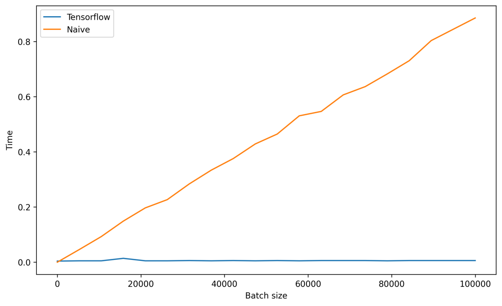
Here one can see particularly well that with increasing the computation time increases linearly for the naive implementation. In contrast, the Tensorflow implementation just requires constant time.

IoU as metric

The IoU function can now be used to evaluate an object localization model. For demonstration purposes, I created a simple toy dataset with rectangles displayed on neutral background (as also described in this post).

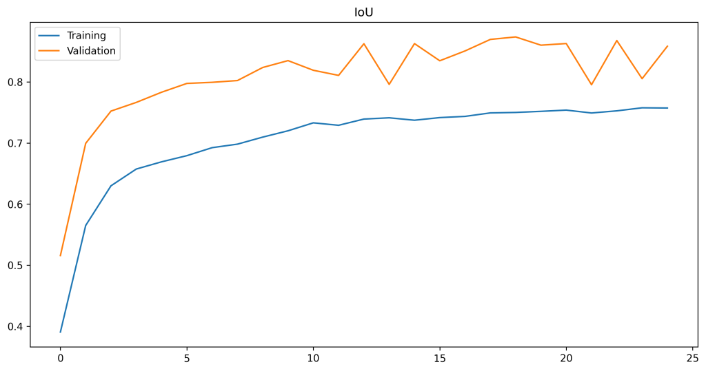
In the compile command you can now pass the IoU function as metric, so that during training, the training and validation IoU is displayed.

model.compile("adam", loss='mse', metrics=IoU)

Epoch 1/25
300/300 [==============================] - 7s 14ms/step - loss: 101.0867 - IoU: 0.3906 - val_loss: 39.8459 - val_IoU: 0.5157
Epoch 2/25
300/300 [==============================] - 4s 14ms/step - loss: 21.8482 - IoU: 0.5650 - val_loss: 8.1091 - val_IoU: 0.6994
Epoch 3/25
300/300 [==============================] - 4s 14ms/step - loss: 11.4204 - IoU: 0.6299 - val_loss: 4.7726 - val_IoU: 0.7522
...

And furthermore, the return value of the fit function contains the history of the IoU over the epochs.

Some examples of the model prediction with the corresponding bounding box:

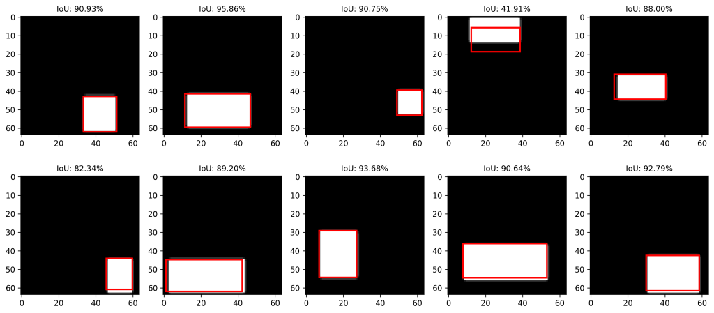
The full code is available here.