In this post I would like to write and give some intuition about the Kullback-Leibler Divergence, which is a measure of how different two probability distributions over the same random variable are. I’ll start by giving an intuitive explanation of the entropy and then derive the Kullback-Leibler Divergence from it. Lastly, I will calculate the KL Divergence for a small toy example.
Self-Information
One of the main goals of information theory is to quantify the information content of data, or in other words, how surprising an event is. For example, consider an unfair coin that lands heads up in 95% of the time. You wouldn’t be surprised if heads are up on a throw. In contrast, you would be very surprised if tails is up.
This intuition, where an unlikely event is more informative than a likely event, is formalized in the Self-Information or Shannon-Information
![]()
which can be rewritten to
![]()
So for our coin example, the probability of heads coming up is ![]() , whereas the probability of tails coming up is
, whereas the probability of tails coming up is ![]() . When calculating the Self-Information for both, we can clearly see that the outcome tails is way more surprising than the outcome heads
. When calculating the Self-Information for both, we can clearly see that the outcome tails is way more surprising than the outcome heads
![]()
![]()
However, usually we are not interested in the surprise of a particular event, but on the surprise we can expect on average for a whole probability distribution. This is where the entropy comes into place.
Entropy
Entropy is the expected value of the Self-Information and is defined for a discrete random variable ![]() with
with ![]() possible values as
possible values as
![]()
One important aspect here is the choice of the logarithm. If it is base 2, the unit of the entropy is in bits. With this in mind, entropy can also be explained as the minimum number of bits (or yes-no-questions) needed, on average, to encode our data.
Consider a fair coin, where each value is equally likely (![]() ). The entropy of one toss would be 1. This indicates, that we need one bit, and thus, one yes-no-question, to encode the data (the bit is either turned on or off).
). The entropy of one toss would be 1. This indicates, that we need one bit, and thus, one yes-no-question, to encode the data (the bit is either turned on or off).
This example can of course be extended to a random variable with multiple possible outcome values. Let’s take a random variable ![]() that can take a value between 1 and 8 (
that can take a value between 1 and 8 (![]() ) each with equal probability
) each with equal probability ![]() . How many yes-no-questions do we need? Calculating the entropy gives us
. How many yes-no-questions do we need? Calculating the entropy gives us
![Rendered by QuickLaTeX.com \[\begin{aligned} H(X) &= - \sum_{i=1}^{8} P(x_i) \cdot \text{log }P(x_i) \\&= - (\frac{1}{8} \cdot \text{log }\frac{1}{8} + … + \frac{1}{8} \cdot \text{log }\frac{1}{8}) \\&= 3 \text{ bits} \end{aligned}\]](https://johfischer.com/wp-content/ql-cache/quicklatex.com-209acac94b6fa54c89c05bf316503ff0_l3.png)
Hence, we need 3 yes-no-questions to find our value, but of course not simply asking “Is the value a 1?”, “Is the value a 2?”, etc. The questions asked are: “Is the value in the first or in the second half?” and that 3 times.
Besides giving a lower bound of the number of bits needed to encode information, entropy is also often given as a measure of the amount of disorder in a system. A high entropy indicates a big amount of disorder, whereas a low entropy indicates a low amount of disorder.
For a better intuition of this notion of entropy, let’s assume a dataset which contains several objects, each belonging to one of two classes. The frequency of class 1 objects can be denoted with the parameter ![]() , so that
, so that ![]() and
and ![]() . In simple terms, if the dataset contains 100 objects and
. In simple terms, if the dataset contains 100 objects and ![]() , then 60 objects belong to class 1 and the rest to class 2.
, then 60 objects belong to class 1 and the rest to class 2.
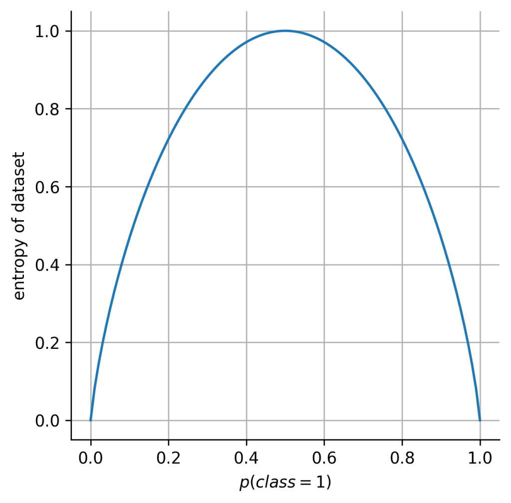
The entropy (or in a loose notion the disorder of the dataset) can then be written as a function of the parameter ![]() :
:
![]()
Note: For those of you who are familiar with machine learning, this equation should already be well-known, as it is nothing more than the binary cross-entropy loss.
Plotting this equation results in the following function:

This plot further visualizes what we’ve discussed so far. If all objects of the dataset belong to only one class (![]() or
or ![]() ) the entropy or disorder of the dataset equals zero. This means loosely spoken, there is “no disorder” in the dataset.
) the entropy or disorder of the dataset equals zero. This means loosely spoken, there is “no disorder” in the dataset.
However, if we are dealing with a balanced dataset (![]() ), the “disorder” is maximal with
), the “disorder” is maximal with ![]() .
.
Note: I have taken a dataset for the example here to illustrate the concept of “disorder”. However, this example can also be rewritten so that it represents the outcome of a Bernoulli random variable with binary outcome: success ![]() or failure
or failure ![]() . This would be more appropriate in terms of entropy being a measure of uncertainty of an outcome, with higher entropy indicating higher uncertainty.
. This would be more appropriate in terms of entropy being a measure of uncertainty of an outcome, with higher entropy indicating higher uncertainty.
Kullback-Leibler Divergence
Up to this point we have seen that self-information is a measure to quantify the information of a specific event, and that the entropy is the expected information for a whole probability distribution. With this we have finally worked out the prerequisites to understand the Kullback-Leibler divergence, which is a measure to quantify how different two distributions are, or in other words, how much information is lost when we approximate one distribution with another.
For two probability distributions ![]() and
and ![]() over the same random variable
over the same random variable ![]() , the Kullback-Leibler Divergence is defined as
, the Kullback-Leibler Divergence is defined as
![Rendered by QuickLaTeX.com \[D_{KL}(P \lVert Q) = \sum_{i=1}^{N} P(x_i) \cdot (\text{log } P(x_i) - \text{log } Q(x_i))\]](https://johfischer.com/wp-content/ql-cache/quicklatex.com-7f15398b3ddc44c6ceb66d937e524a36_l3.png)
which can be rewritten to
![Rendered by QuickLaTeX.com \[D_{KL}(P \lVert Q) = \sum_{i=1}^{N} P(x_i) \cdot \text{log } \frac{P(x_i)}{Q(x_i)}.\]](https://johfischer.com/wp-content/ql-cache/quicklatex.com-f8e80b52e574a1ba839f42a4c8fc2ab8_l3.png)
For a discrete random variable, the KL divergence is the extra amount bits needed to encode samples from ![]() using a code that was designed for samples drawn from
using a code that was designed for samples drawn from ![]() . If both probability distributions are the same, then we would not need any extra bit and thus, the KL-divergence equals zero (the probability distributions do not differ).
. If both probability distributions are the same, then we would not need any extra bit and thus, the KL-divergence equals zero (the probability distributions do not differ).
Intuitive Derivation
For a more intuitive understanding, let’s take the coin example again. Consider a fair coin with equal probability for heads and tails coming up
![]()
and a biased coin where heads is coming up 95% of the time
![]()
One way of comparing these two distributions is to sample some sequences and compare what probability each distribution would assign to each sequence. If both distributions assign similar probabilities to the same sample sequence, it implies that the two distributions might be similar.
Let’s clarify it further with an example, where we draw a sample sequence from the fair coin distribution by tossing the fair coin 10 times. This could generate a sequence like
![]()
with ![]() and
and ![]() .
.
The probability of getting this sequence given the fair coin is
![Rendered by QuickLaTeX.com \[\begin{aligned}P(S_{fair} | \text{ fair coin}) &= P(\text{heads})^{N_{heads}} \cdot P(\text{tails})^{N_{tails}} \nonumber \\&= 0.5^{10}\nonumber \\&\approx 0.001\end{aligned}\]](https://johfischer.com/wp-content/ql-cache/quicklatex.com-e63f2f4792062b2042f0d0eff6f4f141_l3.png)
whereas the probability of generating this sequence when sampling from the biased coin distribution is
![Rendered by QuickLaTeX.com \[\begin{aligned}P(S_{fair} | \text{ biased coin}) &= P(\text{heads})^{N_{heads}} \cdot P(\text{tails})^{N_{tails}} \nonumber \\&= 0.95^{6} \cdot 0.05^{4} \nonumber \\&\approx 0.000005\end{aligned}\]](https://johfischer.com/wp-content/ql-cache/quicklatex.com-422fbcf2eae022cd0f2696e61690415f_l3.png)
When comparing these two probabilities one can clearly see that the likelihood of generating the sequence given the biased coin is way smaller than generating the sequence with the fair coin. This suggests that the two distributions might not be similar, as they assign different probabilities to the same sequence. For a direct comparison we can take the ratio of both probabilities
![]()
as a measure for similarity. Expressing this in a more formal way with
![]() ,
, ![]() for the fair coin and
for the fair coin and
![]() ,
, ![]() for the biased coin gives us
for the biased coin gives us
![Rendered by QuickLaTeX.com \[\frac{P(S_{fair} | \text{ fair coin})}{P(S_{fair} | \text{ biased coin})} = \frac{p_1^{N_{heads}} \cdot p_2^{N_{tails}}}{q_1^{N_{heads}} \cdot q_2^{N_{tails}}}.\]](https://johfischer.com/wp-content/ql-cache/quicklatex.com-8215d685102b316fbf81ec242481fe5b_l3.png)
Taking the log of this equation and normalizing it by the length of the sequence ![]() (sample size) gives us
(sample size) gives us
![Rendered by QuickLaTeX.com \[\frac{1}{N} \cdot \text{log }(\frac{p_1^{N_{heads}} \cdot p_2^{N_{tails}}}{q_1^{N_{heads}} \cdot q_2^{N_{tails}}}).\]](https://johfischer.com/wp-content/ql-cache/quicklatex.com-7e6da360f905d4151961f61d9051e487_l3.png)
By applying logarithm rules we can refine this equation
![Rendered by QuickLaTeX.com \[\begin{aligned}&\frac{1}{N} \cdot \text{log }(\frac{p_1^{N_{heads}} \cdot p_2^{N_{tails}}}{q_1^{N_{heads}} \cdot q_2^{N_{tails}}}) \\ &=\frac{1}{N} \cdot [\text{log }(p_1^{N_{heads}} \cdot p_2^{N_{tails}}) - \text{log }(q_1^{N_{heads}} \cdot q_2^{N_{tails}})] \nonumber \\&= \frac{1}{N} \cdot[\text{log }p_1^{N_{heads}} + \text{log }p_2^{N_{tails}} - \text{log }q_1^{N_{heads}} - \text{log }q_2^{N_{tails}}] \nonumber \\&= \frac{1}{N} \cdot \text{log }p_1^{N_{heads}} +\frac{1}{N} \cdot \text{log }p_2^{N_{tails}} \\& \text{ } -\frac{1}{N} \cdot \text{log }q_1^{N_{heads}} -\frac{1}{N} \cdot \text{log }q_2^{N_{tails}} \nonumber \\&= \frac{{N_{heads}}}{N} \cdot \text{log }p_1 +\frac{{N_{tails}}}{N} \cdot \text{log }p_2 \\ \text{ } &-\frac{{N_{heads}}}{N} \cdot \text{log }q_1 -\frac{{N_{tails}}}{N} \cdot \text{log }q_2\end{aligned}\]](https://johfischer.com/wp-content/ql-cache/quicklatex.com-1fa23fecda6ded2d2a192d67edf44a9a_l3.png)
If the generated sequence from the fair coin is infinitely long the proportion of heads coming up ![]() and the proportion of tails coming up
and the proportion of tails coming up ![]() tends towards
tends towards ![]() and
and ![]() , respectively. Hence,
, respectively. Hence,
![Rendered by QuickLaTeX.com \[\begin{aligned}& \text{ }\frac{{N_{heads}}}{N}\text{log }p_1 +\frac{{N_{tails}}}{N}\text{log }p_2 -\frac{{N_{heads}}}{N}\text{log }q_1 -\frac{{N_{tails}}}{N}\text{log }q_2 \nonumber \\\Leftrightarrow & \text{ }p_1 \text{log }p_1 +p_2 \text{log }p_2 -p_1 \text{log }q_1 -p_2 \text{log }q_2\end{aligned}\]](https://johfischer.com/wp-content/ql-cache/quicklatex.com-462b9c349429d8c5958ce80be8f5c227_l3.png)
Rearranging this equation gives us
![Rendered by QuickLaTeX.com \[\begin{aligned}&p_1 \text{log }p_1 + p_2 \text{log }p_2 -p_1 \text{log }q_1 - p_2 \text{log }q_2\nonumber \\= & p_1 \text{log }p_1 - p_1 \text{log }q_1 + p_2 \text{log }p_2 - p_2 \text{log }q_2\nonumber \\= & \text{ }p_1 (\text{log }p_1 - \text{log }q_1) +p_2 (\text{log }p_2 - \text{log }q_2) \nonumber \\= & p_1 \text{log }\frac{p_1}{q_1} +p_2 \text{log }\frac{p_2}{q_2}\end{aligned}\]](https://johfischer.com/wp-content/ql-cache/quicklatex.com-12927ce72192dc97eb82abc8e268eb1a_l3.png)
which is equivalent to the discrete Kullback-Leibler Divergence
![Rendered by QuickLaTeX.com \[D_{KL}(P \lVert Q) = \sum_{i=1}^{N} P(x_i) \cdot \text{log } \frac{P(x_i)}{Q(x_i)}.\]](https://johfischer.com/wp-content/ql-cache/quicklatex.com-f8e80b52e574a1ba839f42a4c8fc2ab8_l3.png)
Toy Example
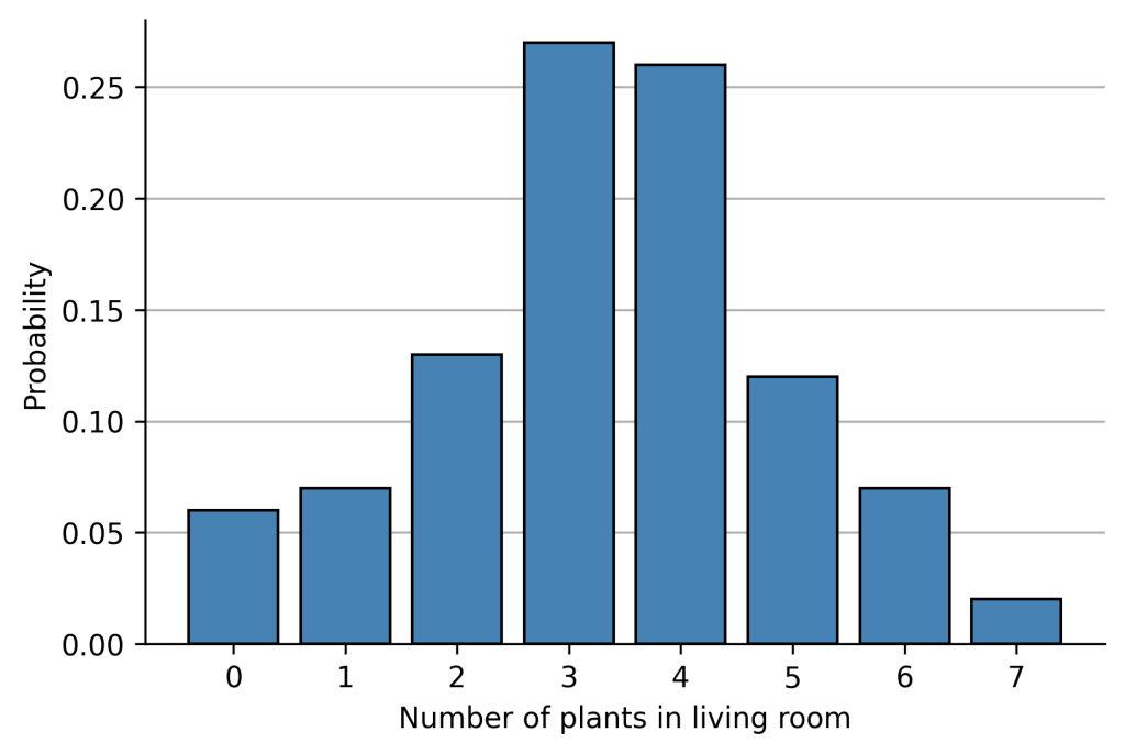
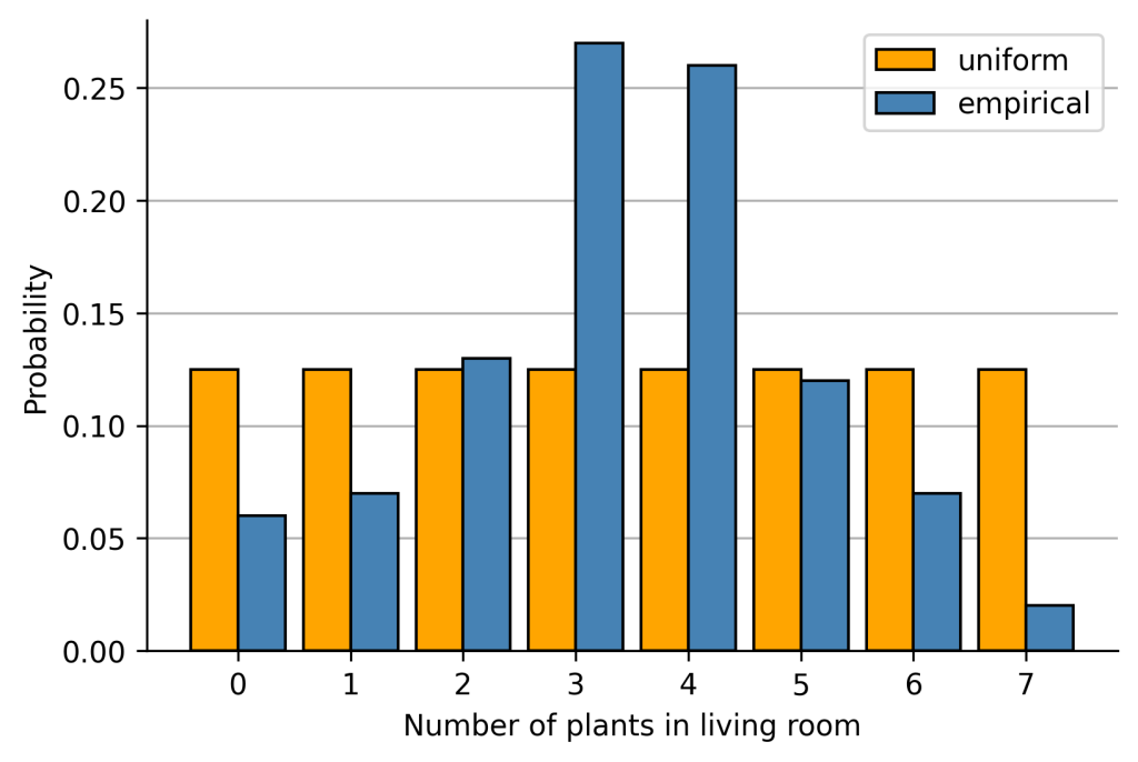
Finally I would like to calculate the Kullback-Leibler Divergence for a small toy example. Assume we conducted a survey where we asked 100 persons how many plants they have in their living room. The empirical probability distribution is

How much information would we lose if we approximate this empirical distribution with a uniform distribution where each outcome is equally likely?

We can calculate that by using the KL divergence with ![]() representing the uniform distribution:
representing the uniform distribution:
![Rendered by QuickLaTeX.com \[\begin{aligned}&D_{KL}(\text{empirical} \lVert \text{uniform}) = \sum_{i=1}^{N} P(x_i) \cdot \text{log } \frac{P(x_i)}{Q(x_i)} \nonumber \\&= P(x=0) \cdot \text{log } \frac{P(x=0)}{Q(x=0)} + … + P(x=7) \cdot \text{log } \frac{P(x=7)}{Q(x=7)} \nonumber \\&= 0.06 \cdot \text{log } \frac{0.06}{0.125} + … + 0.02 \cdot \text{log } \frac{0.02}{0.125} \nonumber \\&\approx 0.341\end{aligned}\]](https://johfischer.com/wp-content/ql-cache/quicklatex.com-c7d25d3a95579a53ec7d7f1a0d07eee4_l3.png)
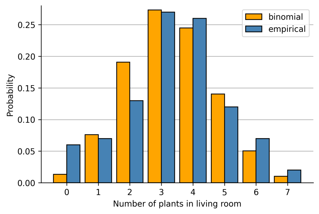
How much information would we lose if we approximate this empirical distribution with a Binomial distribution with parameter ![]() equal to the normalized expectation of our empirical distribution?
equal to the normalized expectation of our empirical distribution?

Again, calculating the Kullback-Leibler divergence with ![]() being the binomial distribution gives us:
being the binomial distribution gives us:
![Rendered by QuickLaTeX.com \[\begin{aligned}&D_{KL}(\text{empirical} \lVert \text{binomial}) =\sum_{i=1}^{N} P(x_i) \cdot \text{log } \frac{P(x_i)}{Q(x_i)}\nonumber \\&= P(x=0) \cdot \text{log } \frac{P(x=0)}{Q(x=0)} + … + P(x=7) \cdot \text{log } \frac{P(x=7)}{Q(x=7)}\nonumber \\&= 0.06 \cdot \text{log } \frac{0.06}{0.013} + … + 0.02 \cdot \text{log } \frac{0.02}{0.01}\nonumber \\&\approx 0.268\end{aligned}\]](https://johfischer.com/wp-content/ql-cache/quicklatex.com-58a6cae9cc9e104aa6c99985023f38a7_l3.png)
By comparing both values we can conclude, that the Binomial distribution approximates our empirical distribution better than the uniform distribution, as the KL divergence is smaller.
Conclusion
Summing up, we have seen that self-information is used to quantify the information of a specific outcome/event and the expected information for a probability distribution is determined by the entropy. The Kullback-Leibler divergence is based on the entropy and a measure to quantify how different two probability distributions are, or in other words, how much information is lost if we approximate one distribution with another distribution.
However, one drawback of the Kullback-Leibler divergence is that it is not a metric, since ![]() (not symmetric). If a symmetric measurement is preferred, I would recommend to read more about the Jensen-Shannon divergence which is bound to values between 0 and 1.
(not symmetric). If a symmetric measurement is preferred, I would recommend to read more about the Jensen-Shannon divergence which is bound to values between 0 and 1.
If you have any comments, feel free to leave a comment below or write a short message. 🙂
References
- Ian J. Goodfellow, Ian J.; Bengio, Yoshua; and Courville, Aaron (2016). Deep Learning. MIT Press.
- Mezard, M., & Montanari, A. (2009). Information, physics, and computation. Oxford University Press.
- Stone, J. V. (2015). Information theory: a tutorial introduction.
Comments are closed, but trackbacks and pingbacks are open.