Denoising Score Matching – Johannes S. Fischer

In the past two years, diffusion models have revolutionized and taken over the field of generative models. In particular, the paper by Ho et al. [1] accelerated this trend. However, in my opinion, one of the most seminal works in this field dates back to 2010 with the technical report of Pascal Vincent [2] that uncovers the link between score matching and denoising autoencoders and derives the denoising-score matching objective. In this blog post I would like to give an intuitive explanation of score-based modeling and introduce the denoising score-matching objective of [2], all accompanied by some visualizations in 1D space.

Generative Modeling

Given data samples $\mathbf{x} = x_1, …, x_n$ drawn from the true data distribution $p(\mathbf{x})$ , in generative modeling we usually try to learn a model that allows us to synthesize new data. While implicit generative models, like Generative Adversarial Networks (GANs), learn the sampling process itself, explicit models try to directly model the probability density function (pdf) in order to sample from this distribution. We can represent such a pdf with an energy-based model

$p_\theta (\mathbf{x}) = \frac{e^{- f_\theta (\mathbf{x})}}{Z_\theta}$

where $\theta$ are the learnable parameters of the model, $Z_\theta$ is a normalizing constant or partition function that ensures that $\int p(\mathbf{x}) \text{ } dx = 1$ , and $f_\theta(\mathbf{x}) \in \mathbb{R}$ is the energy-function or unnormalized probability model, which is usually a deep neural network.

One approach to learning this model would be traditional maximum-likelihood estimation, where we try to find the parameters that maximize the joint density $p_\theta (\mathbf{x}).$ When we insert the energy-based model into the MLE objective we get

$\mathbb{E}_{p(\mathbf{x})}} [- \log p_\theta (\mathbf{x})] = \mathbb{E}_{p(\mathbf{x})} [\log f_\theta (\mathbf{x}) - \log Z_\theta]$

The output of the energy-function or neural network $f_\theta (\mathbf{x})$ is easy to evaluate, however, in order to ensure that the pdf integrates to one, we need to find the normalizing constant $Z_\theta$ , which is usually intractable.

Score Function

Score-based modeling circumvents the problem of finding the normalizing constant $Z_\theta$ by modeling the score function, which is defined as

$s(\mathbf{x}) = \triangledown_{\mathbf{x}} \log p_\theta (\mathbf{x})$

The score is essentially the gradient of the true data log-likelihood evaluated on any point $x$ in data space. Intuitively, given an arbitrary point $x$ , the score at this point tells us in which direction we would need to move to get to a higher density region.

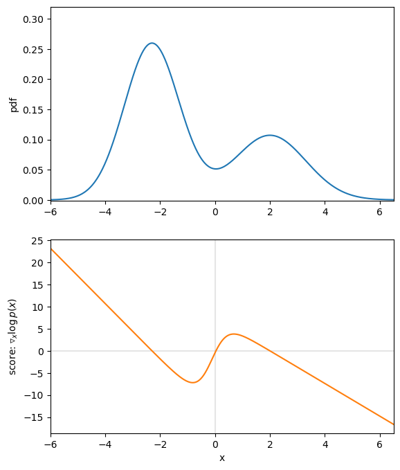
Let’s assume our true data distribution is a simple univariate Gaussian Mixture Model (GMM), as displayed in figure 1. The value of the corresponding score function at each position $x$ , tells us the direction of higher density. For example, if we are at $x = -4$ we can see that the score is positive and thus, if we want to make $x$ slightly more likely under $p(x)$ , we need to move to the right. Contrarily, if we evaluate the point $x = 4$ , the negative score tells us that for a higher density region we need to move to the left.

**Figure 1**: Probability density function of a univariate Gaussian Mixture Model and the corresponding score function.

Score-based model

In order to model the score function, we define a score-based model $s_\theta( \mathbf{x})$ , parametrized by $\theta$ , which tries to approximate the true score function $\triangledown_{\mathbf{x}} \log p(\mathbf{x})$ . If we insert the definition of the energy-based model and apply the logarithm quotient rule we get

$\begin{aligned}s_\theta (\mathbf{x})&= \triangledown_{\mathbf{x}} \log p_\theta(\mathbf{x}) \\&= \triangledown_{\mathbf{x}} \log \frac{e^{- f_\theta (\mathbf{x})}}{Z_\theta} \\&= \triangledown_{\mathbf{x}} \log e^{- f_\theta (\mathbf{x})} - \underbrace{\triangledown_{\mathbf{x}} \log Z_\theta}_{=0} \\&= - \triangledown_{\mathbf{x}} f_\theta (\mathbf{x})\end{aligned}$

With that we can see that our score-based model is independent of the normalizing constant $Z_\theta$ , as the gradient w.r.t. the input $x$ develops to zero. Hence, in contrast to MLE, we model an unconstrained function without the need for normalization. Intuitively, instead of learning the pdf with the corresponding partition function, our model learns some kind of navigation map that, at every point $x$ in data space, leads us to higher density regions.

Training this model then just breaks down to a simple regression problem known as score-matching, where $s_\theta (\mathbf{x})$ should learn to best match the gradient of the true log likelihood at every point $x$ . The objective can be defined as the Euclidean distance (Fisher divergence) between the true score and our score-based model

$\begin{aligned}J(\theta)&= \mathbb{E}_{p(\mathbf{x})} [\lVert s_\theta (\mathbf{x}) - s(\mathbf{x})\rVert^2_2] \\&= \mathbb{E}_{p(\mathbf{x})} [\lVert s_\theta (\mathbf{x}) - \triangledown_{\mathbf{x}} \log p(\mathbf{x})\rVert^2_2]\end{aligned}$

However, this objective brings up two problems. First, it requires us to have access to the true score of the data distribution, which we usually don’t have. And second, it fails to learn good estimates of the score in low density regions, as we weight it with $p(x)$ when we evaluate the expectation $\mathbb{E}_{p(\mathbf{x})}$ .

The paper of Vincent [2] addresses both of these problems by linking score matching to the Denoising Autoencoder objective.

Denoising Score-Matching

The general goal of Denoising Autoencoders is to learn a model that denoises a corrupted sample $\tilde{x}$ to get back to the original sample $x$ .

We can easily create a perturbed version of our original dataset by simply adding Gaussian noise, controlled by the variance $\sigma^2$ , to each data sample s.t. the corrupted version of $\mathbf{x}$ is defined as $\tilde{\mathbf{x}} = \mathbf{x} + \epsilon$ with $\epsilon \sim \mathcal{N}(0, \sigma^2 \cdot \mathbf{I})$ .

**Figure 2**: Probability density function of the original univariate Gaussian Mixture Model and the corrupted version for different variance scales.

Defining the explicit score-matching objective for the corrupted dataset $q_\sigma (\tilde{\mathbf{x}})$ yields

$\begin{aligned}J_{explicit}(\theta) = \mathbb{E}_{q_\sigma (\tilde{\mathbf{x}})}[ \frac{1}{2}\lVert s_\theta (\tilde{\mathbf{x}}) -\triangledown_{\tilde{\mathbf{x}}} \log q_\sigma (\tilde{\mathbf{x}})\rVert^2_2].\end{aligned}$

So far we still cannot evaluate the score. However, in an elegant proof in the appendix of the original paper [2], Vincent shows that this objective can be considered as equivalent to the following denoising score matching (DSM) objective

$\begin{aligned}J_{DSM_\sigma}(\theta) =\mathbb{E}_{q_\sigma (\tilde{\mathbf{x}}, \mathbf{x})}[ \frac{1}{2} \lVert s_\theta (\tilde{\mathbf{x}}) -\triangledown_{\tilde{\mathbf{x}}} \log q_\sigma (\tilde{\mathbf{x}} | \mathbf{x})\rVert^2_2]\end{aligned}$

over the joint density $q_\sigma (\tilde{\mathbf{x}}, \mathbf{x}) = q_\sigma (\tilde{\mathbf{x}} | \mathbf{x}) p(\mathbf{x})$ .

While $\triangledown_{\tilde{\mathbf{x}}} \log p_\sigma (\tilde{\mathbf{x}})$ is a complex distribution and we thus cannot evaluate it, $p_\sigma(\tilde{\mathbf{x}} | \mathbf{x})$ follows a normal distribution $\mathcal{N}(\mathbf{x}, \sigma^2 \cdot \mathbf{I})$ with mean $\mathbf{x}$ and variance $\sigma^2$ , as

$\tilde{\mathbf{x}} = \mathbf{x} + \epsilon \iff \tilde{\mathbf{x}} \sim \mathcal{N}(\mathbf{x}, \sigma^2 \cdot I)$

with $\epsilon \sim \mathcal{N}(0, \sigma^2 \cdot \mathbf{I})$ (see Convolution of probability distributions).

This allows us to easily derive the gradient

$\begin{aligned}\triangledown_{\tilde{\mathbf{x}}} \log q_\sigma (\tilde{\mathbf{x}} | \mathbf{x})&= \triangledown_{\tilde{\mathbf{x}}} \log \mathcal{N}(\mathbf{x}, \sigma^2 \cdot \mathbf{I})\\&= \triangledown_{\tilde{\mathbf{x}}} \log \frac{\exp(-\frac{1}{2} (\tilde{\mathbf{x}} - \mathbf{x})^T \cdot (\sigma^2 \cdot \mathbf{I})^{-1} \cdot(\tilde{\mathbf{x}} - \mathbf{x}))}{\sqrt{(2\pi)^d | \sigma^2 \cdot \mathbf{I} |}}\\&= \triangledown_{\tilde{\mathbf{x}}}\log \exp(-\frac{1}{2} (\tilde{\mathbf{x}} - \mathbf{x})^T\cdot (\sigma^2 \cdot \mathbf{I})^{-1} \cdot(\tilde{\mathbf{x}} - \mathbf{x}))\\ & \hspace{0.8cm} - \underbrace{\triangledown_{\tilde{\mathbf{x}}} \log \sqrt{(2\pi)^d | \sigma^2 \cdot \mathbf{I} |}}_{= 0} ]\\&= -\frac{1}{2\sigma^2} \triangledown_{\tilde{\mathbf{x}}}(\tilde{\mathbf{x}} - \mathbf{x})^T \cdot \mathbf{I} \cdot (\tilde{\mathbf{x}} - \mathbf{x})\\&= -\frac{1}{2\sigma^2} \triangledown_{\tilde{\mathbf{x}}} (\tilde{\mathbf{x}} - \mathbf{x})^2\\&= - \frac{(\tilde{\mathbf{x}} - \mathbf{x})}{\sigma^2} = \frac{(\mathbf{x} - \tilde{\mathbf{x}})} {\sigma^2}.\end{aligned}$

Intuitively, the gradient corresponds to the direction of moving from $\tilde{\mathbf{x}}$ back to the original $\mathbf{x}$ (i.e., denoising it), and we want our score-based model $s_\theta (\tilde{\mathbf{x}})$ to match that as best as it can.

Figure 3 visualizes that for the 1D case. We can see that the direction of the denoising score $\triangledown_{\tilde{\mathbf{x}}} \log q_\sigma (\tilde{\mathbf{x}} | \mathbf{x})$ almost perfectly matches the direction of the ground truth score $\triangledown_{\mathbf{x}} \log p (\mathbf{x})$ . Thus, we found an appropriate target for our score-matching objective, so that we can learn the score function.

**Figure 3:** Probability density function of the original univariate Gaussian Mixture Model and the corrupted version for $\sigma^2 = 0.6$ , with corresponding scores. Arrows indicate the direction of the ground truth and denoising score for different values of $x$ .

**Figure 3:** Probability density function of the original univariate Gaussian Mixture Model and the corrupted version for $\sigma^2 = 0.6$ , with corresponding scores. Arrows indicate the direction of the ground truth and denoising score for different values of $x$ .

Conclusion

With the denoising score matching objective we are able to circumvent the problem of not having access to the true score of our data distribution and additionally, with larger noise scales, also get signals in low density regions.

On a first glance it seems like there exists a trade-off between small versus large additive noise scales $\sigma^2$ . With small noise scales the denoising score approximates the ground truth score well, but we cannot cover much of the low density regions, whereas with larger noise scales we can cover more of the low density regions, but our targets are less accurate, as they may not match the actual score anymore.

However, as we can easily generate different noisy versions of our dataset, we can sidestep this problem by simply using multiple noise scales. Intuitively, we populate the whole data space with a large noise scale, s.t. in low density regions we get a rough direction in which to move. Then, iteratively, we decrease our noise scale and get a finer and finer direction towards regions with higher density. This is exactly what happens in Denoising Diffusion Probabilistic Models (DDPM) [1]. Visually speaking, DDPMs learn a navigation map in data space that guides them to the actual data manifold.

References

[1] Ho, J., Jain, A., & Abbeel, P. (2020). Denoising diffusion probabilistic models. Advances in Neural Information Processing Systems, 33, 6840-6851.

[2] Vincent, P. (2011). A connection between score matching and denoising autoencoders. Neural computation, 23(7), 1661-1674.

[3] Song, Y. (2021). Blog “Generative Modeling by Estimating Gradients of the Data Distribution”. https://yang-song.net/blog/2021/score/.