This project was done for the Mobile Robotics course in the Intelligent Interactive Systems master’s program at Pompeu Fabra University, Barcelona.
In the following I will give a short overview of how I approached the task of implementing a localization module and present the results. The code for this project can be found here.
Environment
For the environment I have chosen Gazebo simulation, where I made up my own room in which a robot must localize itself using landmarks. These landmarks were distributed in the corners of the room and represented by cubes or spheres. The position of the landmarks was given to the robot in advance.
For the robot I decided to go with Tiago robot (PAL Robotics – Titanium), which is a two wheeled robot with one arm. However, the arm was neglected for the purpose of this project.
Sensor model
For the distance from the robot to the different landmarks I used the Euclidean distance. The model consists of an artificial GPS which sends noisy estimation of the distance to the landmarks. For simplicity I used the ground truth odometry and added randomly generated normally distributed noise.
Movement
The robot was able to move forward, as well as to rotate, either in the left or right direction.
Motion Model
As the movement of the robot was given in distance units and turn units (radiant), the robots position was set as follows. First, the orientation of the robot was set, by adding the desired turn in radiant to the current orientation. To limit the values of the orientation to be within the range -π to π, an orientation over π was projected to negative π plus the delta between π and the orientation, and vice versa. Second, the distance was set and new values were computed for x and y, respectively. This was done by using the unit circle, where x + cos(angle) * distance leads to the new x value and y + sin(angle) * distance to the new y value. The robot’s position was set to these new values only if they were valid.
Localization Module
For this project I wanted to implement a particle filter. To achieve this, I used multiple classes:
Robotclass which included all the movement, and sensing functions, and as properties the estimated and true pose (x, y, orientation), the world settings (size, landmarks) and the GPS and sensing noise.Particleclass, which included movement and sensing as the robot, but without actually moving the robot. Furthermore it included a weighting function, that weighted the particle according to the measurements (distance to landmarks).ParticleFilterclass which was the parent class of the Particle class and included the world settings, an array of particles which were initialized when a new ParticleFilter was created, the weights of the particles (initialized with
  for each particle) and functions to simulate the motion of all particles, weight them, resample particles based on their weight, estimate the robots position based on the particles, and lastly, visualize the current situation.
main_localizationscript that combined all classes and ran the localizationutilclass with helper functions, e.g. computing the distance, a gaussian function, limiting function, conversion function from quaternions to Euler angles, function to compute the mean of circular quantities, a normalization function, and theVelMsgclass which initialized a Twist message with all values being zero, and setter function for either the forward movement or rotationWorldclass where the landmarks and the size of the world was stored
As a first step of localization, a world object was created using an array of landmarks, and the size of the world. Then a ParticleFilter object was created, which had as arguments the number of particles, the noise for moving a particle forward, turning it, or for its sensing, and the world object. Thereafter a rospy node and the robot were initialized and the loop for the particle filter was started. In each iteration, the robot was moved, either randomly or with a fixed pattern (both can be seen in the video). Then the robots motion was simulated for each particle, which was achieved in the same way the robots motion was conducted, but without moving the robot.
In a second step the particles got weighted based on their agreement with the current measurements of the robot, and then normalized, so they sum up to one in the end.
The third step was to resample the particles, but with higher weighted particles being drawn more often than particles with less weight. Finally the robots position got estimated based on the particles. I used the weighted mean for all particles to estimate x and y, and the mean of circular quantities for the orientation.
Results
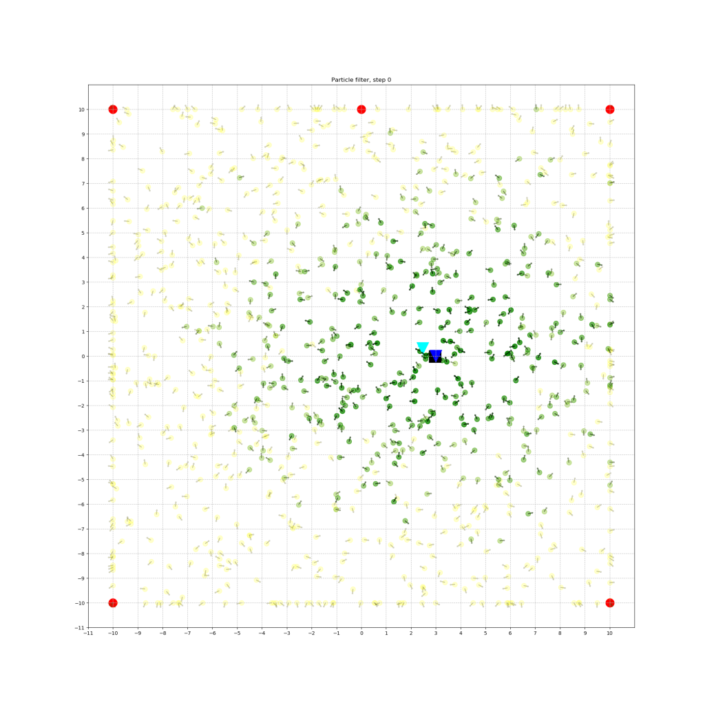
In the beginning the particles were distributed uniformly across the map, as it can be seen in the figure below.

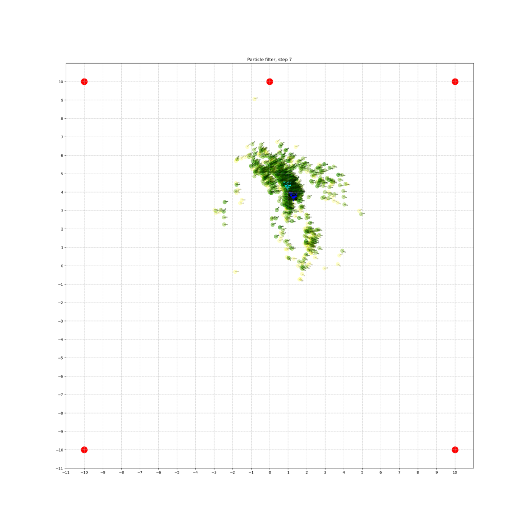
Yellow particles represent the initial particles, and green particles display the resampled ones. The true position of the robot is visualized with a black square, the robots position based on the motion model with a cyan triangle, and the estimate of the position based on the particles with a blue triangle. Red symbolize the landmarks that were given to the robot in advance.
With increasing time and hence, more movement, the particles position and orientation slowly converge to be closer to the ground truth. This is further illustrated in the figure below.

If you have any questions or comments, feel free to leave a reply here or write an email. 🙂
The Github-Repo can be found here: https://github.com/joh-fischer/robot-localization
Comments are closed, but trackbacks and pingbacks are open.