Object Detection Part 2: Localization and Classification

Simple object localization and classification using a convolutional neural network build with Tensorflow/Keras in Python.

In my previous post I wrote about a simple object localization problem: predicting the bounding box of a single rectangle on neutral background. However, this approach was limited to a single shape and could not distinguish multiple shapes. In this post I will tackle this problem by extending the previous model, so that it is able to also classify the objects’ shape.

To do so, I will create a simple toy dataset and build a simple CNN with two heads: a regression head for the bounding box prediction, and a classification head for the shape recognition.

The Task

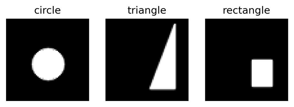
The input of the network is a $n \times n$ image with black background, displaying one of three shapes: a rectangle, a circle, or a triangle. For simplicity I decided to use gray scale images, instead of colored ones.

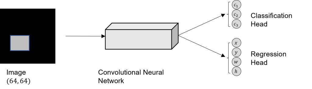
There are two major goals for the network: Localizing the object and classifying the shape. The localization happens by predicting the bounding box of the shape which has the form $(x, y, w, h)$ , with $(x, y)$ being the coordinates of the top-left corner, and $w$ and $h$ are the width and height, respectively. For the classification a one-hot encoding vector will be used. So the final target vector has the shape $(c_1, c_2, c_3, x, y, w, h)$ , where the first three positions are responsible for classifying the shape (rectangle, circle, triangle), and the last four for predicting the bounding box.

Create Dataset

As in the previous post, I will create the dataset by myself using numpy and OpenCV. Visualization is done using matplotlib. The images will have a shape of $64 \times 64$ , and each object has a minimum pixel size of $12$ . Per class, 10.000 images will be created.

import numpy as np
import matplotlib.pyplot as plt
import cv2

n_samples_per_class = 10000
image_size = 64
min_size = 12

The creation of the rectangles is pretty straightforward. First, an image array with dimension $(64, 64, 1$ is created, where $1$ corresponds to the color channel (gray = 1). Then $x$ , $y$ , $w$ , and $h$ are generated randomly, respecting the minimum size. Thereafter, OpenCV’s $rectangle$ function is used to add the rectangle to the black image array. The function returns the image, as well as the target vector, which consists of the one-hot encoding of the classification $[1, 0, 0]$ , indicating that the shape is a rectangle, and the corresponding bounding box values $[x, y, w, h]$ .

def create_rectangleXY(img_size, min_obj_size):
    x_rect = np.zeros((img_size, img_size, 1), dtype="uint8")
    
    # get random top-left corner
    x, y = np.random.randint(0, img_size - min_obj_size, 2)
    
    # get random width and height
    w = np.random.randint(min_obj_size, img_size - x)
    h = np.random.randint(min_obj_size, img_size - y)
    
    color = np.random.randint(150, 255, dtype=int)
    cv2.rectangle(x_rect, (x, y), (x+w,y+h), color, -1, lineType=cv2.LINE_AA)
    
    return x_rect, [1, 0, 0, x, y, w, h]

The circle image is generated similarly, but instead of generating random width and height, generating the radius randomly.

def create_circleXY(img_size, min_obj_size):
    x_circle = np.zeros((img_size, img_size, 1), dtype="uint8")
    
    # get random radius
    radius = np.random.randint(min_obj_size // 2, img_size // 2)
    
    # get random top-left corner
    x, y = np.random.randint(radius, img_size - radius, 2)
    
    color = np.random.randint(150, 255, dtype=int)
    cv2.circle(x_circle, (x, y), radius, color, -1, lineType=cv2.LINE_AA)
    
    return x_circle, [0, 1, 0, x-radius, y-radius, radius*2, radius*2]

Lastly, we need a function to create triangles. This is done by generating random $x$ , $y$ , $w$ , and $h$ , with which the four points of a rectangle can be created. Then one of these four points is randomly deleted, and the remaining three points are used as corners for the triangle.

def create_triangleXY(img_size, min_obj_size):
    x_triangle = np.zeros((image_size, image_size, 1), dtype="uint8")
    
    # get random top-left corner 
    x, y = np.random.randint(0, image_size - min_size, 2)
    
    # get random width and height
    w = np.random.randint(min_size, image_size - x)
    h = np.random.randint(min_size, image_size - y)
    
    # create all four points from x,y,w,h
    pts = [(x,y), (x+w, y+h), (x+w, y), (x, y+h)]
    
    # select 3 points as edges for the triangle
    pts.pop(np.random.randint(0, len(pts)-1))
    
    color = np.random.randint(150, 255, dtype=int)
    cv2.drawContours(x_triangle, [np.array( pts )], 0, color, -1,
                     lineType=cv2.LINE_AA)
    
    return x_triangle, [0, 0, 1, x, y, w, h]

Now we can put everything together and create our dataset as follows.

np.random.seed(280295)

X = []
Y = []
for i in range(n_samples_per_class):
    # rectangle image
    x_rect, y_rect = create_rectangleXY(image_size, min_size)
    X.append(x_rect)
    Y.append(y_rect)
    
    # circle image
    x_circle, y_circle = create_circleXY(image_size, min_size)
    X.append(x_circle)
    Y.append(y_circle)
    
    # triangle image
    x_triangle, y_triangle = create_triangleXY(image_size, min_size)
    X.append(x_triangle)
    Y.append(y_triangle)

X = np.array( X )
Y = np.array( Y )

print("X: ", X.shape)  # (30000, 64, 64, 1)
print("Y: ", Y.shape)  # (30000, 7)

For later we will also implement a function that translates the one-hot encoding vector into a written label. E.g., $[1, 0, 0] \rightarrow$ rectangle.

LABELS = ['rect', 'circle', 'triangle']

def onehot2label(onehot_vec):
    return LABELS[np.argmax(onehot_vec)]

Now let’s display some of our data to see if it worked out properly.

plt.figure(figsize=(12, 5))
for i in range(10):
    ax = plt.subplot(2, 5, i+1)
    plt.imshow(X[i], "gray")
    plt.title(onehot2label(Y[i, :3]) )
plt.show()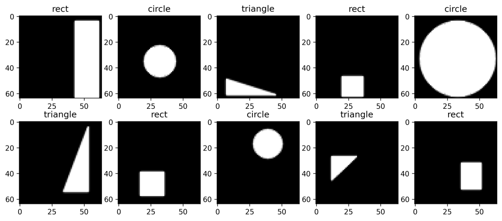

Prepare Data

In image processing it is common to normalize the pixel value to be centered around 0, which I will do by dividing the image values by 255 (the maximum RGB value) and subtracting 0.5. Furthermore, I will shuffle the data, as currently the samples are ordered.

from sklearn.utils import shuffle

# normalize and center pixel values
X = (X.astype("float32") / 255 ) - 0.5

X, Y = shuffle(X, Y)

The next step is to split the dataset into training, validation, and test set.

from sklearn.model_selection import train_test_split

X_train_val, X_test, Y_train_val, Y_test = train_test_split(X, Y, test_size=0.2)

# further split train_val
X_train, X_val, Y_train, Y_val = train_test_split(X_train_val, Y_train_val, test_size=0.2, random_state=29)

print("Shape X train:\t  ", X_train.shape)  # (19200, 64, 64, 1)
print("Shape X validate: ", X_val.shape)    # (4800, 64, 64, 1)
print("Shape X test:\t  ", X_test.shape)    # (6000, 64, 64, 1)

Convolutional Neural Network

The networks goal is to predict the bounding box, as well as the class of an object. Hence, we have a regression, as well as a classification problem. For regression problems, the Mean Squared Error is generally an appropriate loss function, whereas for classification tasks, it is often better to use the categorical cross-entropy.

Furthermore, it is common to use a Softmax activation function for classification since this transforms the output into a probability distribution, where each output is in the range $[0, 1]$ and all outputs add up to 1.

$softmax(y_i) = \frac{e^{y_i}}{\sum_{j=1}^{n} e^{y_j}}.$

Hence, to have both, a classification and a regression output, we need to split the networks output into two heads. The architecture is then as follows:

Network architecture with regression and classification head.

For the two heads of the network (regression and classification) we need to split the target vector $Y$ .

Y_train_split = (Y_train[:, :3], Y_train[:, 3:])
Y_val_split = (Y_val[:, :3], Y_val[:, 3:])
Y_test_split = (Y_test[:, :3], Y_test[:, 3:])

Now it’s time to build the final model. This network is no linear stack of layers, this is why we need to use the Tensorflow functional API, which allows to implement two output heads.

from tensorflow.keras.layers import Conv2D, MaxPooling2D, Dense
from tensorflow.keras.layers import Flatten, Dropout
from tensorflow.keras import Input, Model

inputs = Input(shape=(image_size, image_size, 1))
x = Conv2D(16, kernel_size=(3,3), activation="relu")(inputs)
x = MaxPooling2D(pool_size=(2,2))(x)
x = Conv2D(32, kernel_size=(3,3), activation="relu")(x)
x = MaxPooling2D(pool_size=(2,2))(x)
x = Flatten()(x)
x = Dropout(0.5)(x)
class_out = Dense(3, activation="softmax", name="class")(x)
bbox_out = Dense(4, name="bbox")(x)

model = Model(inputs=inputs, outputs=(class_out, bbox_out))

As you can see in this code block, we first create a simple linear stack of convolutional and max-pooling layers that convolve the image. Then, the input gets flattened and a dropout layer is added to prevent overfitting. Now comes the tricky part. The output of the dropout layer is fed into both, the dense layer for classification, with Softmax activation, and the dense layer for regression. To better visualize what has happened let’s plot the model.

from tensorflow.keras.utils import plot_model

plot_model(model, "./blog images/model_regAndClassHead.png", show_shapes=True)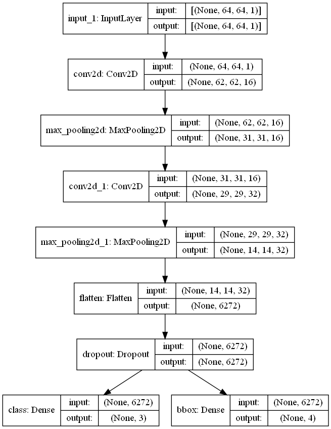

Model architecture with input/output shapes.

One can now clearly see that the output of the dropout layer is fed to both, the classification and the regression head.

Time to compile the model.

model.compile("adam", loss=['categorical_crossentropy', 'mse'],
              metrics=["accuracy"])

I use the Adam Optimizer and two different Losses, one for each head. The classification head is trained using the categorical cross-entropy loss and the regression head with the Mean Squared Error.

It’s time to train the model. Here it’s important to pass the split version of the target vector $Y$ .

%%time
epochs = 35
history = model.fit(X_train, Y_train_split,
                    epochs=epochs,
                    validation_data=(X_val, Y_val_split))

Training the model for 35 epochs on my setup (GPU: Nvidia GeForce GTX 1050 Ti, CPU: Intel i5-3470) takes about 3 minutes and 57 seconds.

Results

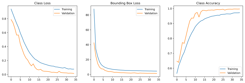
When evaluating the history of the training process one can see how the losses of both heads decrease, and the classification accuracy increases over time.

Loss for both heads over epochs, as well as classification accuracy over epochs.

Let’s evaluate the model on (unseen) test data.

metrics = model.evaluate(X_test, Y_test_split)
for i, name in enumerate(model.metrics_names):
    print(name.replace("_", " ") + ":\t%.4f" % metrics[i])

# OUTPUT
# loss:	    1.3797
# class loss:	0.0173
# bbox loss:	1.3624
# class accuracy:	0.9960
# bbox accuracy:	0.9470

In classification the model performs quite well, with a loss of $0.0173$ and $99.6$ % accuracy. But truth be told, this task is not too difficult to learn for the network. 😉

But also the Mean Squared Error Loss for the bounding box regression seems good. Again, as mentioned in the previous post, the accuracy for the bounding box regression is not a good evaluation metric. The mean Intersection over Union is a better measure of accuracy here.

Note: If you don’t know what the Intersection over Union is, I would recommend to read this post.

# predict test set
preds = model.predict(X_test)

# compute mean IoU
mean_IoU = IoU(Y_test_split[1], preds[1])
print("Mean IoU: %.2f%%" % (mean_IoU*100))

# Mean IoU: 84.84%

A mean Intersection over Union of $82.35%$ is not too bad. Let’s visualize some examples of our test set:

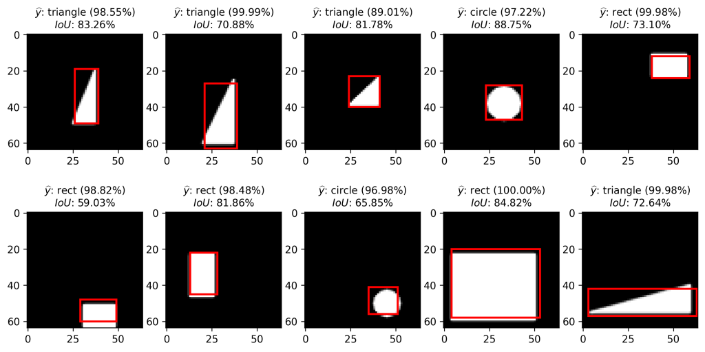
Resulting bounding box predictions and the corresponding classification confidence, as well as the IoU.

Each of the shapes was correctly recognized and every bounding box predicted relatively accurately.

Conclusion

In this blog post we build a simple convolutional neural network that is able to localize and classify a shape on a neutral background. For that we separated the networks head into a bounding box regression and classification head.

However, there is still the drawback that the model can only classify and localize one object per image. How can we classify and localize several objects in an image? In the next post I will try to tackle this problem and build a model that can detect several shapes in an image.

If you have any comments or doubts about what I’ve done so far, feel free to leave a comment or write a mail. 🙂

Github Repo