Including feature selection methods as a preprocessing step in predictive modeling comes with several advantages. It can reduce model complexity, enhance learning efficiency, and can even increase predictive power by reducing noise.
In this blog post I want to introduce a simple python implementation of the correlation-based feature selection algorithm according to Hall [1]. First, I will explain the general procedure. Thereafter I will show and describe how I implemented each step of the algorithm. And lastly, I will proof its functionality by applying it on the Madelon feature selection benchmark dataset. This dataset represents a binary classification problem with 500 continuous features and 2600 samples.
General Principle
The correlation-based feature selection (CFS) method is a filter approach and therefore independent of the final classification model. It evaluates feature subsets only based on data intrinsic properties, as the name already suggest: correlations.
The goal is to find a feature subset with low feature-feature correlation, to avoid redundancy, and high feature-class correlation to maintain or increase predictive power.
For that, the algorithm estimates the merit of a subset  with
with  features with the following equation:
 .
.
 : average feature-feature correlation
 : average feature-class correlation
- : number of features of that subset
For this blog post the features are continuous and hence, we can use the standard Pearson correlation coefficient for the feature-feature correlation. However, as the class of the dataset is binary, the feature-class correlation is computed using the Point-biserial correlation coefficient.
It’s obvious that we search for the subset that yields the highest merit. A high merit can be achieved with a high feature-class correlation in the numerator, as well as with a low feature-feature correlation in the denominator. But how do we search for the best subset?
Imagine a dataset with only 10 features. There are about  possible feature subset combinations and adding one single feature to the dataset would even double the possibilities. Hence, a Brute-Force approach is not really applicable.
Hall (2000) proposes a best first search approach using the merit as heuristic. The search starts with an empty subset and evaluates for each feature the merit of being added to the empty set. For this step the feature-feature correlation can be neglected, as the denominator of the equation above simplifies to 1, due to  .
.

So for the first iteration the evaluation is solely based on the feature-class correlation. The feature with the highest feature-class correlation is added to the so far empty subset. In the next step again all features, except for the one already added, are evaluated and the one that forms the best subset with the previously added one is kept.
This process is iterative and whenever an expansion of features yields no improvement, the algorithm drops back to the next best unexpanded subset. Without a limitation this algorithm searches the whole feature subset space. Hence, the number of backtracks must be limited. After reaching this limit the algorithm returns the feature subset that yielded the highest merit up to this point.
Implementation
Firstly, we will load the dataset with pandas from the drive:
import pandas as pd

# load the dataset
df = pd.read_csv('./data/madelon.csv')
df.head(3)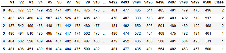
Before we dive deeper into the correlation-based feature selection we need to do some preprocessing of the dataset. First, we want to get the column names of all features and the class, respectively. Second, the class labels are currently 1 and 2. We quickly want to change it to 0 and 1 using numpy’s where function.
import numpy as np

# name of the label (can be seen in the dataframe)
label = 'Class'

# list with feature names (V1, V2, V3, ...)
features = df.columns.tolist()
features.remove(label)

# change class labeling to 0 and 1
df[label] = np.where( df[label] > 1, 1, 0)
Compute Merit
Now we are ready to go to the actual feature selection algorithm. The first thing to implement is the evaluation function (merit), which gets the subset and label name as inputs.
from scipy.stats import pointbiserialr
from math import sqrt

def getMerit(subset, label):
    k = len(subset)

    # average feature-class correlation
    rcf_all = []
    for feature in subset:
        coeff = pointbiserialr( df[label], df[feature] )
        rcf_all.append( abs( coeff.correlation ) )
    rcf = np.mean( rcf_all )

    # average feature-feature correlation
    corr = df[subset].corr()
    corr.values[np.tril_indices_from(corr.values)] = np.nan
    corr = abs(corr)
    rff = corr.unstack().mean()

    return (k * rcf) / sqrt(k + k * (k-1) * rff)
Calculating the average feature-class correlation is quite simple. We iterate through all features in the subset and compute for each feature its Point-biserial correlation coefficient using scipy’s pointbiserialr function. As we are only interested in the magnitude of correlation and not the direction we take the absolute value. Thereafter we take the average over all features of that subset which is our .
For the average feature-feature correlation it get’s a little bit more complicated. We first do the correlation matrix of the subset. Let’s assume our subset includes the first 4 features (V1, V2, V3, V4). We compute the correlation matrix as follows:
subset = ['V1', 'V2', 'V3', 'V4']
corr = df[subset].corr()
corr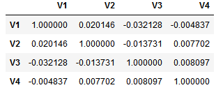
This results in a correlation matrix with redundant values as it is symmetrical and the correlation of each feature with itself is of course 1. Hence, we need to mask redundant values.
corr.values[np.tril_indices_from(corr.values)] = np.nan
corr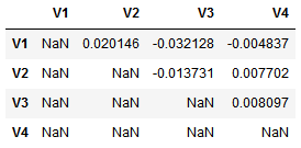
Now we can just unstack the absolute values and take their mean. That’s it!
Best First Search
As already described above, the search starts with iterating through all features and searching for the feature with the highest feature-class correlation.
best_value = -1
best_feature = ''
for feature in features:
    coeff = pointbiserialr( df[label], df[feature] )
    abs_coeff = abs( coeff.correlation )
    if abs_coeff > best_value:
        best_value = abs_coeff
        best_feature = feature

print("Feature %s with merit %.4f"%(best_feature, best_value))

# Output: Feature V476 with merit 0.2255
The best first feature is the one with name V476, as it has the highest feature-class correlation. For the following best first search iterations we need a priority queue as data structure. Each item in this queue has a priority associated with it and at request the item with the highest priority will be returned. In our case the items are feature subsets and the priorities are the corresponding merits. For example, the subset with just the feature V476 has the merit 0.2255. The implementation is quick and dirty for this blog, but of course it could be enhanced, for example using heap sort etc.
class PriorityQueue:
    def  __init__(self):
        self.queue = []

    def isEmpty(self):
        return len(self.queue) == 0

    def push(self, item, priority):
        """
        item already in priority queue with smaller priority:
        -> update its priority
        item already in priority queue with higher priority:
        -> do nothing
        if item not in priority queue:
        -> push it
        """
        for index, (i, p) in enumerate(self.queue):
            if (set(i) == set(item)):
                if (p >= priority):
                    break
                del self.queue[index]
                self.queue.append( (item, priority) )
                break
        else:
            self.queue.append( (item, priority) )

    def pop(self):
        # return item with highest priority and remove it from queue
        max_idx = 0
        for index, (i, p) in enumerate(self.queue):
            if (self.queue[max_idx][1] < p):
                max_idx = index
        (item, priority) = self.queue[max_idx]
        del self.queue[max_idx]
        return (item, priority)
Now we are prepared for the actual search. We first initialize a priority queue and push our first subset containing just one feature (V476).
# initialize queue
queue = PriorityQueue()

# push first tuple (subset, merit)
queue.push([best_feature], best_value)
For the search we need a list of already visited nodes (subsets), a counter for the number of backtracks, and the maximum number of backtracks, as otherwise the search algorithm would search the whole feature subset space.
# list for visited nodes
visited = []

# counter for backtracks
n_backtrack = 0

# limit of backtracks
max_backtrack = 5
The search algorithm works as follows: In the beginning only one feature is in the subset. The algorithm expands this subset with all other possible features and looks for the feature that increases the merit the most. For example, we have the feature V476 in our subset. Now every feature is added to the subset and the merit of it evaluated. So the first expansion is the subset (V476, V1), then (V476, V2), then (V476, V3), and so on. The subset that achieves the highest merit is the new base set and again all features are one by one added and the subsets are evaluated.
# repeat until queue is empty
# or the maximum number of backtracks is reached
while not queue.isEmpty():
    # get element of queue with highest merit
    subset, priority = queue.pop()

    # check whether the priority of this subset
    # is higher than the current best subset
    if (priority < best_value):
        n_backtrack += 1
    else:
        best_value = priority
        best_subset = subset

    # goal condition
    if (n_backtrack == max_backtrack):
        break

    # iterate through all features and look of one can
    # increase the merit
    for feature in features:
        temp_subset = subset + [feature]

        # check if this subset has already been evaluated
        for node in visited:
            if (set(node) == set(temp_subset)):
                break
        # if not, ...
        else:
            # ... mark it as visited
            visited.append( temp_subset )
            # ... compute merit
            merit = getMerit(temp_subset, label)
            # and push it to the queue
            queue.push(temp_subset, merit)
After a few minutes we get the subset that achieves the highest merit, which consists of 48 features. Compared to 500 this is a reduction of around 90%. Not bad!
But how does the subset perform compared to a model with all features?
Validation
To proof the functionality we will use a Support Vector Machine (SVM) for classification. We train one model with all features and compare it to a model using just the subset.
The first SVM we train takes all features as input.
from sklearn.model_selection import cross_val_score
from sklearn import svm
import time

# predictors
X = df[features].to_numpy()
# target
Y = df[label].to_numpy()

# get timing
t0 = time.time()

# run SVM with 10-fold cross validation
svc = svm.SVC(kernel='rbf', C=100, gamma=0.01, random_state=42)
scores = cross_val_score(svc, X, Y, cv=10)
best_score = np.mean( scores )

print("Score: %.2f%% (Time: %.4f s)"%(best_score*100, time.time() - t0))

# Output
# Score: 50.00% (Time: 40.1259 s)
Now we compare it to a SVM that uses only the subset selected by the Correlation-based feature selection algorithm.
# predictors
X = df[best_subset].to_numpy()

# get timing
t0 = time.time()

# run SVM with 10-fold cross validation
svc = svm.SVC(kernel='rbf', C=100, gamma=0.01, random_state=42)
scores_subset = cross_val_score(svc, X, Y, cv=10)
best_score = np.mean( scores_subset )

print("Score: %.2f%% (Time: %.4f s)"%(best_score*100, time.time() - t0))

# Output
# Score: 66.50% (Time: 5.8936 s)
Conclusions
The Correlation-based feature selection algorithm according to Hall [1] was able to significantly reduce the number of features from 500 to 48, which reduced training and evaluation time drastically from 40 to just about 6 seconds. More importantly, this preprocessing step increased accuracy from 50% to about 66.5% with 10-fold cross-validation.
These results confirm that feature selection methods are an appropriate tool to decrease model complexity and are able to boost model performance.
References
[1] Hall, M. A. (2000). Correlation-based feature selection of discrete and numeric class machine learning.
Comments are closed, but trackbacks and pingbacks are open.