Class Activation Maps – Johannes S. Fischer

A method to visualize internal representations of a convolutional neural network and perform object localization without bounding box annotations.

For a university project we investigated the question of where a deep convolutional neural network (CNN) looks, when classifying emotions. For this purpose, we evaluated three visualization methods for CNNs, one of which, the simplest, I would like to share in this post.

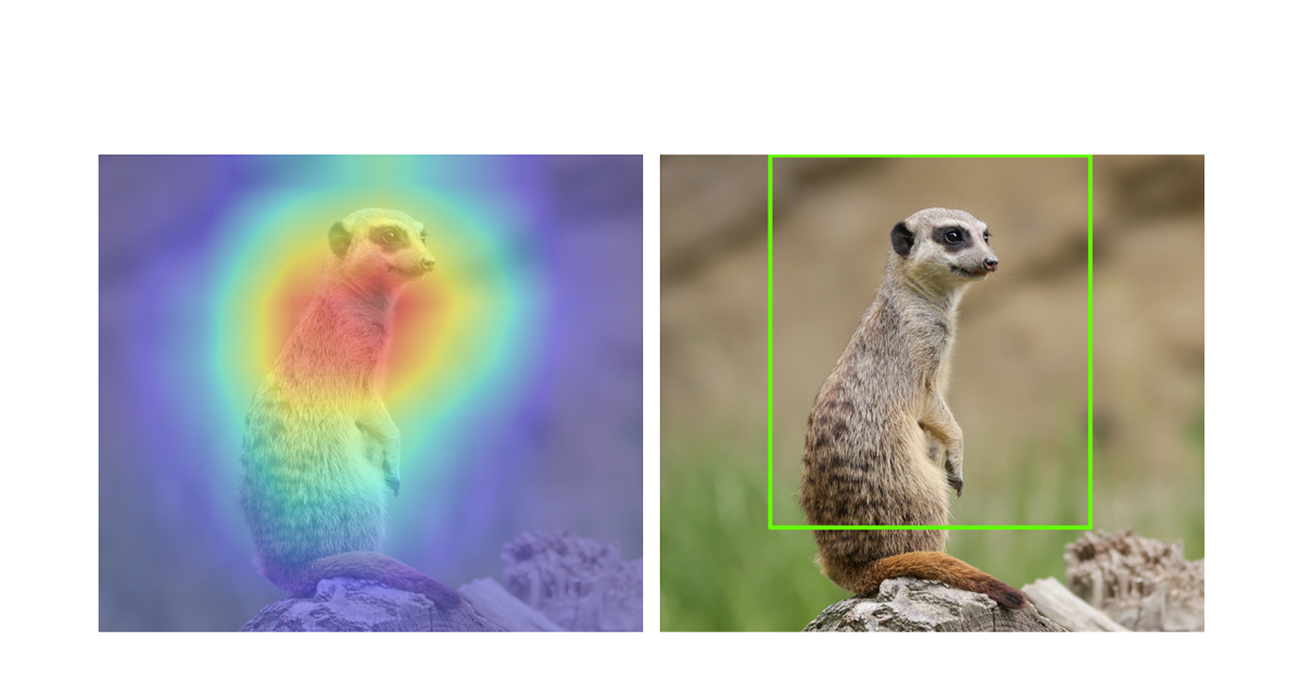
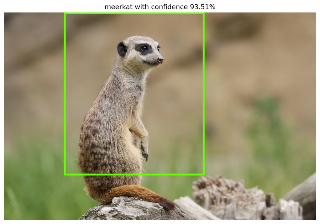
The method is called Class Activation Mapping and was introduced in the paper Learning Deep Features for Discriminative Localization by Zhou et al. (2016) [5]. Besides proposing a method to visualize the discriminative regions of a classification-trained convolutional neural network (CNN), the authors also use this method to localize objects without providing the model with any bounding box annotations. The model just learns the classification task with class labels and is then able to localize the object of a specific class in an image. The result can look like this:

The original image, the class activation map, and the bounding box.

In this post I will first introduce the approach and then present a simple implementation of it in Tensorflow.

Introduction

When training a CNN several filters are learned for convolution operations and each filter application results in a feature map. Filters close to the input layer of a CNN are often detecting low-level features, such as edges or lines. The deeper you go, the more are those low-level features combined into higher level features.

Taking a network where the last convolutional layer is right before the classification layer (softmax), the feature maps can even correspond to objects that are classified with the CNN [5]. For example, let’s take any neural network that is able to classify a person, as well as a dog. The figure below displays such a network with corresponding activations of the feature maps of the last convolutional layer.

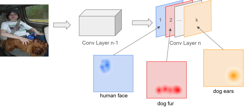
Each feature map of the last convolutional layer focuses on detecting one concept. Feature map 1 in the network above might detect human faces, whereas feature map 2 is responsible for detecting the fur of a dog and feature map k is responsible for detecting the ears of a dog. The combination of several concepts then forms an object.

The authors of [5] even increased the interpretability of the feature maps, as the number of feature maps of the last convolutional layer in their network was equal to the number of classes. Hence, each feature map could be interpreted as confidence map for a specific class. The strongest activation of a class specific feature map was then roughly at the same region as the object was in the original image.

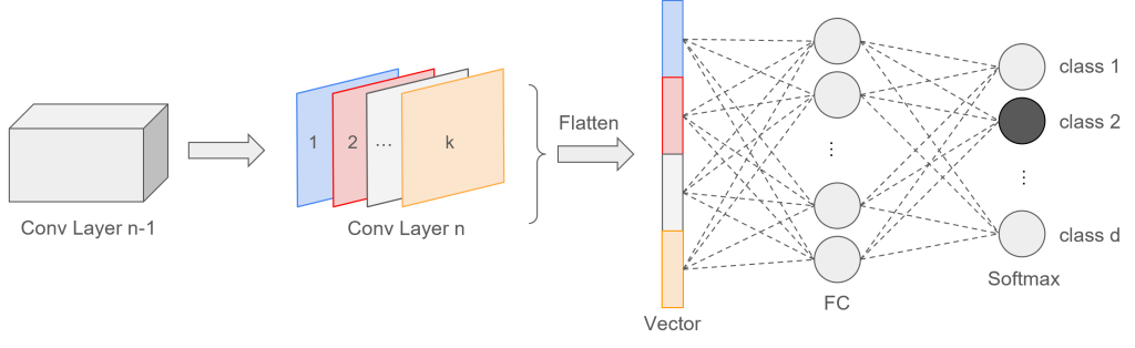
With the normal approach of flattening the feature maps in order to feed them into fully-connected (FC) layers, this direct correspondence between the feature maps and the output gets lost, as the FC layers act like a black box between them [5].

Standard approach, where the feature maps are flattened in order to fed them into a dense layer.

Some recent CNNs, such as the Network in Network [1] or members of the GoogLeNet [3, 4] family, therefore try to avoid the use of FC layers. Instead of flattening the input, [1] proposed to use global average pooling, which maintains the correspondence and keeps the localization ability of the network.

Global average pooling just takes the spatial average over of each of the $k$ feature maps and creates a vector with $k$ scalar values, each representing the mean activation of a feature map.

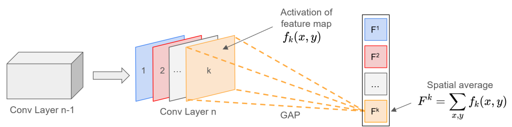
The resulting vector can then be fed into a classification (softmax) layer, so that the activation of a specific class output $S_c$ is just a linear combination of average feature map activations multiplied by the weights corresponding to class $c$ .

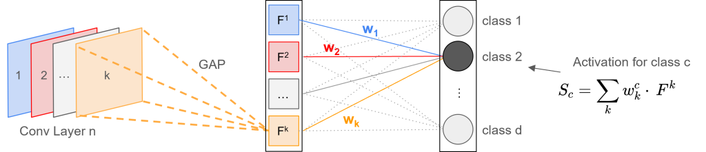
For an illustrative example, let’s assume that we are interested in finding a dog in an image. The activation for the classification layer with respect to the class dog is

$S_{dog} = w_1^{dog} \cdot F^1 + w_2^{dog} \cdot F^2 + ... + w_k^{dog} \cdot F^k$

where $w_i^c$ are the weights for the global average of feature map $i$ with respect to the class $c$ , and $F^i$ are the feature maps of the last conv layer.

When feeding an image of a dog in the network, the convolutions in the last convolutional layer detect some concepts belonging to the class dog, for example, the ears and the body. The feature maps that are responsible for detecting those concepts will have a high activation, and hence, also the spatial averages $F^i$ of those feature maps will be high.

The weights $w_i^c$ indicate the importance of feature map $F^i$ for class $c$ . For the dog example this means, that weights combining the concepts (feature maps) belonging to the class dog, might have a higher value than weights that are associated with feature maps that do detect other concepts, that are not important for the class dog.

Class Activation Mapping

Zhou et al. (2016) [5] use this property of networks with global average pooling to identify the most discriminative regions of an image by combining a linear weighted sum of the feature maps. So instead of multiplying the weights with the global averages of the feature maps, the authors propose to directly multiply the feature maps with the weights corresponding to the class.

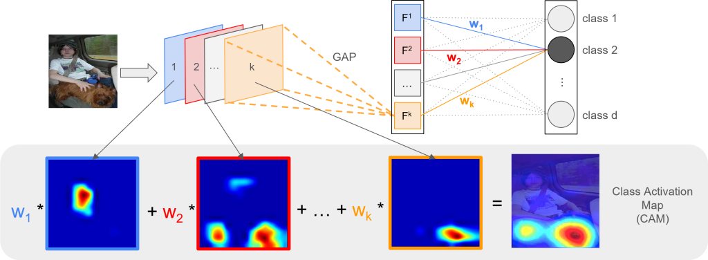
Linear combination of the weights and feature maps to obtain the class activation map.

The result of the linear combination of weights and feature maps is called Class Activation Map (CAM) and perfectly highlights the regions of an image that are important for discrimination. Loosely speaking, you can say that it indicates where the network is looking when predicting a certain class. Mathematically this is defined as

$M_c(x,y) = \sum_k w_k^c \cdot f_k(x,y)$

with $M_c(x,y)$ being the activation of pixel $(x, y)$ of class $c$ , which is the linear combination of the weights $w_k^c$ for each feature map multiplied by the pixel $(x, y)$ in each feature map. Hence, the CAM is just a weighted linear sum of the presence of specific visual patterns at different spatial locations.

To further understand the concept, we will implement the method in simple python code.

Implementation

Let’s first import the required packages.

import numpy as np
import tensorflow as tf
import cv2
import matplotlib.pyplot as plt

# pretrained inception model
import tensorflow.keras.applications.inception_v3 as inception_v3

As the use of Class Activation Maps proposed by this paper is restricted to networks with global average pooling layers directly before the softmax classification layer, I will use the InceptionV3 network [4] which is a revised version of the GoogLeNet network.

# load model
model = inception_v3.InceptionV3(weights='imagenet')

The image for classification is the following, which I just downloaded from the internet.

IMG_NAME = 'meerkat.jpg'
img = plt.imread(IMG_NAME)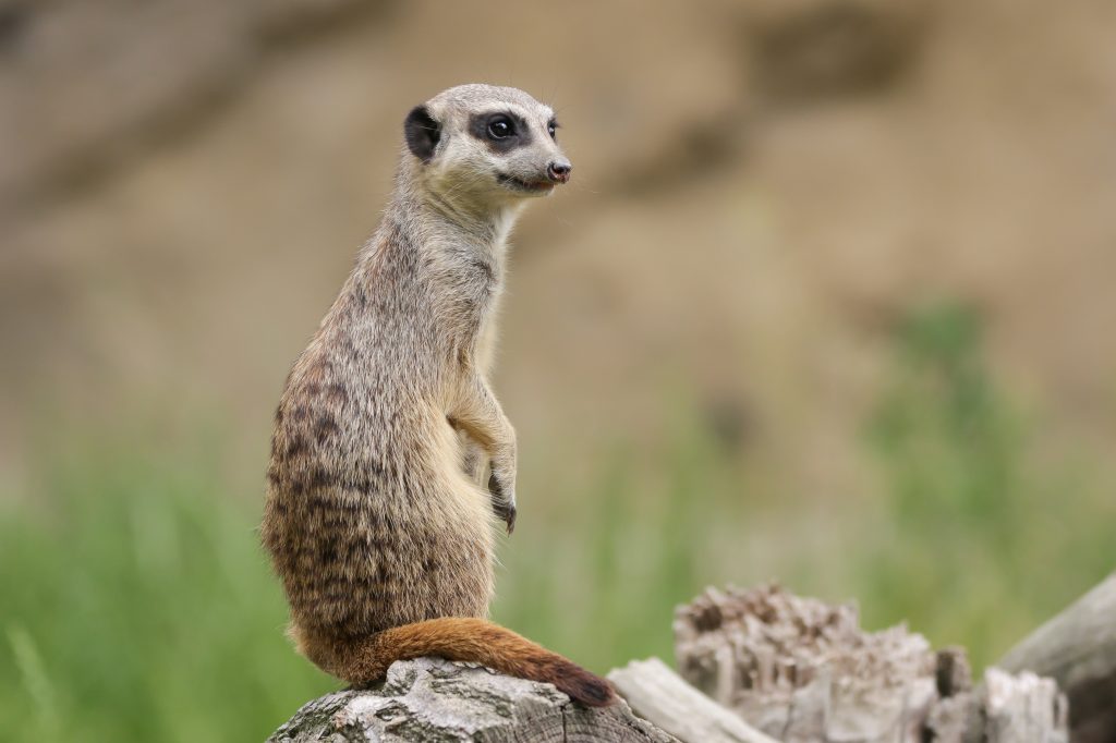

For the inception network the image needs to have a specific size ( $299 \times 299$ ), therefore we need to resize it. Furthermore, we need to make a batch out of it (expand the dimensions so that is has shape (1, 299, 299, 3)) and preprocess it. The tensorflow inception module provides us a function for that, which converts the images from RGB to BGR and then zero-centers each color channel with respect to the ImageNet dataset.

x = cv2.resize(img, (299, 299))
x = np.expand_dims(x, axis=0) 
x = inception_v3.preprocess_input(x)

Let’s see what the model predicts for our image.

preds = model.predict(x)

preds_decoded = inception_v3.decode_predictions(preds)[0]

_, label, conf = preds_decoded[0]
print("Label: %s with confidence %.2f%%" % (label, conf*100))

# OUTPUT: Label meerkat with confidence 93.51%

We can see that the model is able to correctly classify the image. So now let’s go to the actual CAM algorithm.

Class Activation Map

The general steps to obtain the Class Activation Map (CAM) are as follows:

Get the feature maps of the last conv layer
Get the weights connecting the global average pooling layer with the specific class of the softmax layer
Multiply each feature map with the corresponding weight to obtain the Class Activation Map

For the first step we have to take a look at the model summary to identify the name of the layer that is directly before the global average pooling layer.

model.summary()

From the output we can see that the layer we are searching for is called mixed10. With that information we can build a new model that, besides outputting the classification, also gives us the activations of the feature maps for a specific input image.

last_conv_layer = model.get_layer('mixed10')

model_fm = tf.keras.Model(inputs=model.inputs,
                          outputs=[
                              model.output,
                              last_conv_layer.output
                          ])

When we now feed the image in the altered model, we get both, the feature maps, as well as the prediction.

model_out, feature_maps = model_fm.predict(x)

# get rid of the batch channel, e.g. (1, 1000) -> (1000,)
feature_maps = np.squeeze(feature_maps)
model_out = np.squeeze(model_out)

print(model_out.shape)        # (1000,)
print(feature_maps.shape)     # (8, 8, 2048)

The last convolutional operation outputs 2048 feature maps, each with a size of $8 \times 8$ . Next, we need to get the weights connecting the GlobalAveragePooling layer with the softmax classification layer. For now we are only interested in the weights for the winning class. Hence, we need to find the index of the class with highest confidence.

# get weights of last layer
weights = model.layers[-1].weights[0]
print(weights.shape)       # (2048, 1000)

# find winning class (highest confidence)
max_idx = np.argmax( model_out )
print(f"Max index: {max_idx} ({model_out[max_idx]*100:.2f}%)")
# OUTPUT: Max index = 299 (93.51%)

The weights matrix has shape $n_F \times n_c$ where $n_F$ is the number of feature maps (or number of outputs of the global average pooling layer) and $n_c$ is the number of classes the model is able to predict.

$\mathbf{W} = \begin{pmatrix} w_{11} & ... & w_{1 n_c} \\ \vdots & \ddots & \vdots \\ w_{n_F 1} & ... & w_{n_F n_c}\end{pmatrix}$

As we only need the weights of the winning class, we can just take the column of the winning class (max_idx) of the matrix above.

winning_weights = weights[:, max_idx]
print(winning_weights.shape)    # (2048,)

As expected, the weight vector has exactly the same number of rows, as we have feature maps in the last layer. So for each feature map we have one corresponding weight. With the notion of feature maps as concept learners, we could say that each weight determines how important the specific concept is for the output/class.

Now we only need to scale each feature map with the corresponding weight. For example, for feature map $k$ which has dimensions $(8 \times 8)$ , we multiply each pixel with the scalar value $w_k$ .

We could write that in really simple python code:

CAM = np.zeros(feature_maps.shape[:2])
for k, wk in enumerate(winning_weights):
    # get feature map k
    feature_map_k = feature_maps[..., k]
    
    # get activation of map k (multiply Fk with wk)
    activation_k = feature_map_k * wk
    
    CAM += activation_k

However, this method is quite slow. A faster and nicer way is to use numpy’s functionality of multiplying matrices.

CAM = np.sum(feature_maps * winning_weights, axis=2)

When plotting the result we get the following heatmap:

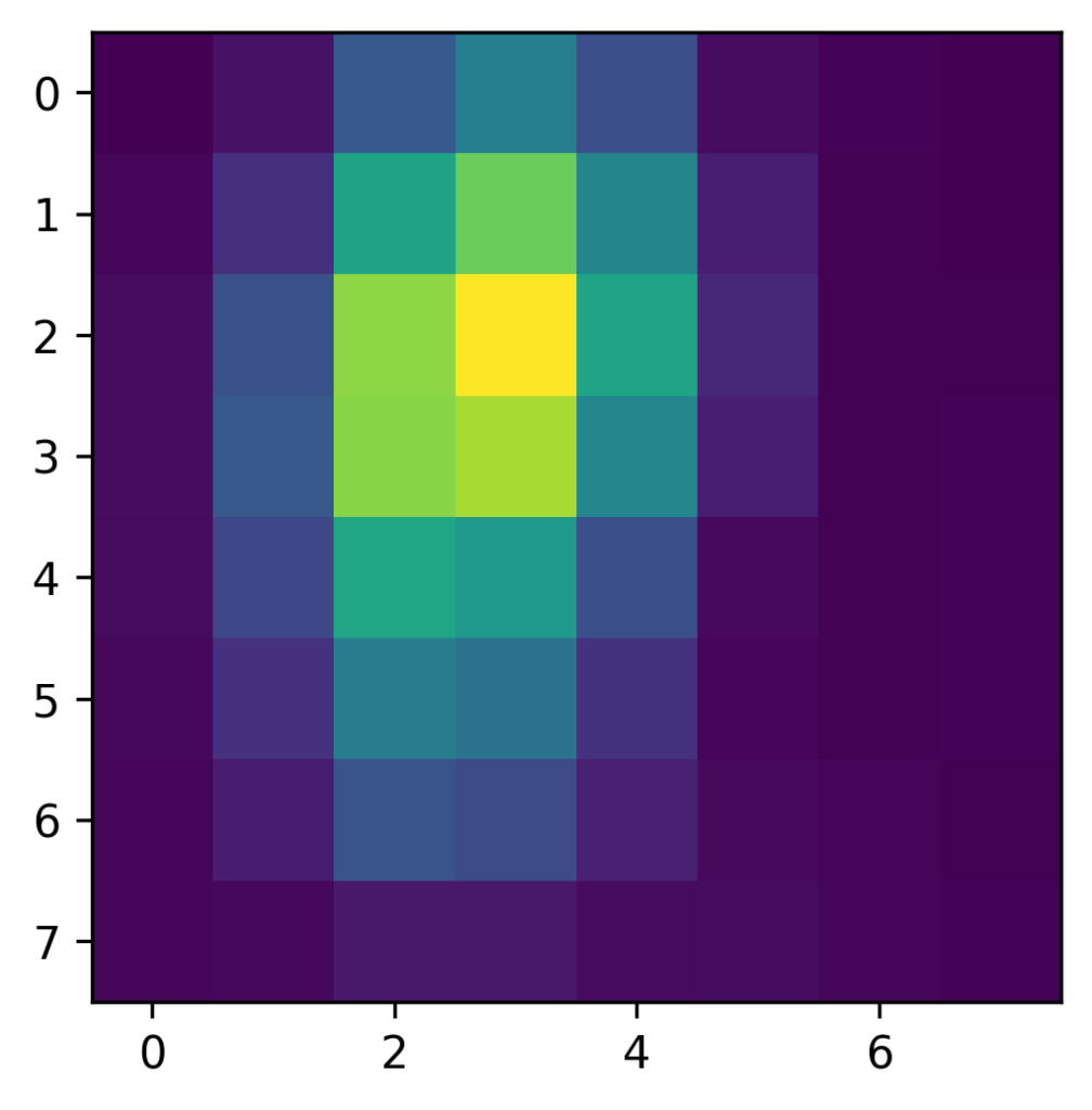
Class Activation Map for the meerkat image.

This looks quite good so far! However, this heatmap is really small, as it only has the dimensions of the feature maps in the last conv layer ( $8 \times 8$ ). To nicely plot it and compare it to our input image, we need to upscale the Class Activation Map to the size of our image.

# resize CAM
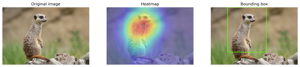
heatmap = cv2.resize(CAM, (img.shape[1], img.shape[0]))

Plotting the heatmap and the original image size by side we get:

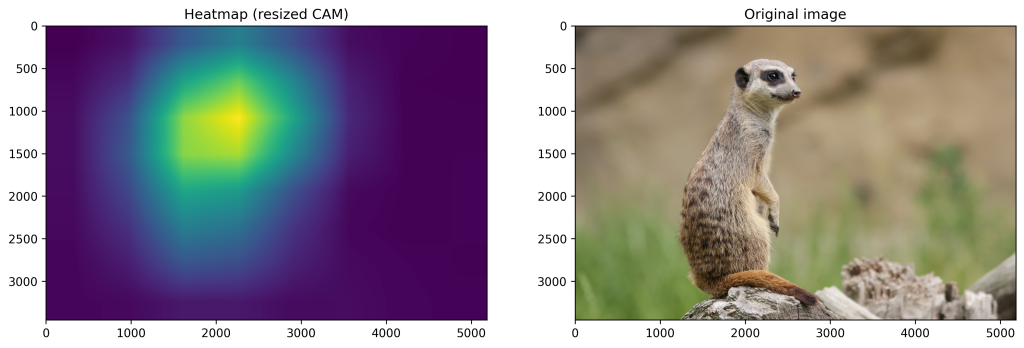
Now if we superimpose the heatmap over the image, we get a pretty good visualization of the regions that are important for the network to identify the meerkat.

Heatmap superimposed over the original image.

In order to perform localization and generate a bounding box for the class, the authors propose a simple thresholding technique [5]. They first segment the regions where the value is above 20% of the max value of the Class Activation Map and then take the bounding box that covers the largest connected component in the segmentation map.

That’s how the visualization of discriminative regions and weakly-supervised localization works with Class Activation Mapping. 🙂

Conclusion

Class Activation Maps are a useful tool to visualize class-discriminative regions of a deep convolutional neural network. With simple techniques one can obtain a heatmap for these regions and furthermore, use this heatmap to localize an object and draw a bounding box around it. Hence, the method allows to learn an object localization task solely by using class labels instead of bounding box annotations.

However, the Class Activation Mapping approach is quite limited in the sense, that it can only be applied to models having a certain architecture. The model needs to have a global average pooling layer right after the last convolutional layer, followed by the classification layer. A newer and more flexible approach, called GradCAM [2] overcomes this limitation by using gradients flowing back from the classification output to the feature maps of the last convolutional layer. This makes the approach somehow independent of the architecture and allows the application to most neural network architectures. In some future post I am planning to write about GradCAM as well. 🙂

Lastly, I would like to show a small result of our university project. We trained several CNNs on different datasets for emotion recognition and then evaluated different visualization techniques to find out what regions are important to recognize a certain emotion. This is one result we obtained with CAM:

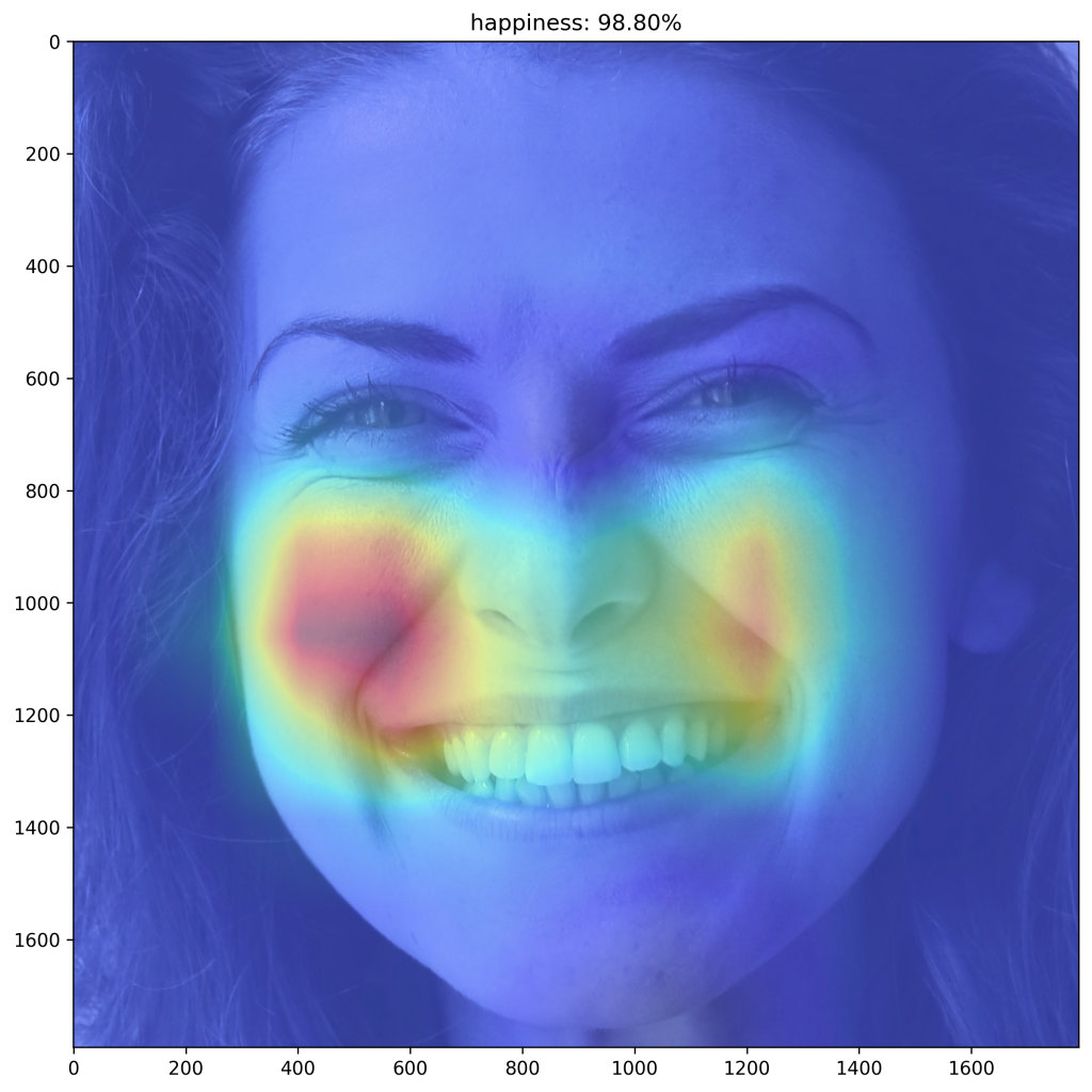
It seems like the laugh lines play a special role in classifying happy people. 😉

References

[1] Lin, M., Chen, Q., & Yan, S. (2013). Network in network. arXiv preprint arXiv:1312.4400.

[2] Selvaraju, R. R., Cogswell, M., Das, A., Vedantam, R., Parikh, D., & Batra, D. (2017). Grad-cam: Visual explanations from deep networks via gradient-based localization. In Proceedings of the IEEE international conference on computer vision (pp. 618-626).

[3] Szegedy, C., Liu, W., Jia, Y., Sermanet, P., Reed, S., Anguelov, D., … & Rabinovich, A. (2015). Going deeper with convolutions. In Proceedings of the IEEE conference on computer vision and pattern recognition (pp. 1-9).

[4] Szegedy, C., Vanhoucke, V., Ioffe, S., Shlens, J., & Wojna, Z. (2016). Rethinking the inception architecture for computer vision. In Proceedings of the IEEE conference on computer vision and pattern recognition (pp. 2818-2826).

[5] Zhou, B., Khosla, A., Lapedriza, A., Oliva, A., & Torralba, A. (2016). Learning deep features for discriminative localization. In Proceedings of the IEEE conference on computer vision and pattern recognition (pp. 2921-2929).

—

If you have any comments or questions, feel free to leave a reply below or write an email. The code to this post can be found on my github.