Object Detection Part 1: Localization

Simple introduction to object localization using a convolutional neural network build with Tensorflow/Keras in Python.

In the past days I worked myself into object detection with neural networks. For simplicity, I decided to start with a simple task: predict the bounding box of one single rectangle on a neutral background. This has the advantages that I can generate the data set myself and the training is not as costly as with normal images.

So let’s dive into it! 🙂

The Task

The network gets as input a $n \times n$ image with black background and a green rectangle and will predict the target vector $(x, y, w, h)$ , where x and y denote the top-left corner of the rectangle and $w$ and $h$ are the width and height of it, respectively. This is further illustrated in the following image, with $n=8$ :

Example image of size 8 and green rectangle at position (2, 2).

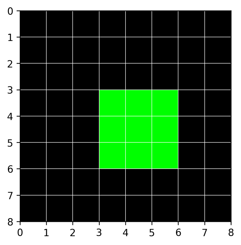
The target rectangle starts at position $x=2$ and $y=2$ and has a width and height of $3$ . Hence, the algorithm should predict $(2, 2, 3, 3)$ .

As the task is clear now, let’s start with creating the toy dataset!

Create Dataset

With an image size of 8 the possibilities for a rectangle would be quite limited. Therefore, I decided to set the size to 64, which easily allows to draw 40.000 samples. The minimum size for the rectangle is set to 8. I will use standard libraries, such as numpy, pyplot, and OpenCV.

import numpy as np
import matplotlib.pyplot as plt
import cv2

# dataset settings
n_samples = 40000
image_size = 64
min_size = 8

The images will be stored in a numpy array $X$ with the dimensions (40000, 64, 64, 3), where 40.000 refers to the number of images, 64 to the image width and height, and 3 to the number of color channels (RGB). The target vector for one image has four elements (x, y, width, height). Thus, $Y$ has the dimensions (40000, 4).

X = np.zeros((n_samples, image_size, image_size, 3), dtype="uint8")
Y = np.zeros((n_samples, 4))

The creation of the images works as follows:

for sample in range(n_samples):
    # create image
    img = np.zeros((image_size, image_size, 3), dtype="uint8")
    
    # get random x and y coordinate
    x = np.random.randint(0, image_size - min_size)
    y = np.random.randint(0, image_size - min_size)
    
    # get random width and height
    w = np.random.randint(min_size, image_size - x)
    h = np.random.randint(min_size, image_size - y)

    # assign target vector to sample
    Y[sample] = [x, y, w, h]

    # draw rectangle on image
    cv2.rectangle(img, (x,y), (x+w,y+h), (0, 255, 0), -1)
    X[sample] = img

To inspect what we’ve done so far, lets plot the first 10 images:

plt.figure(figsize=(12, 4))
for i in range(10):
    plt.subplot(2, 5, i+1)
    plt.imshow(X[i])
plt.show()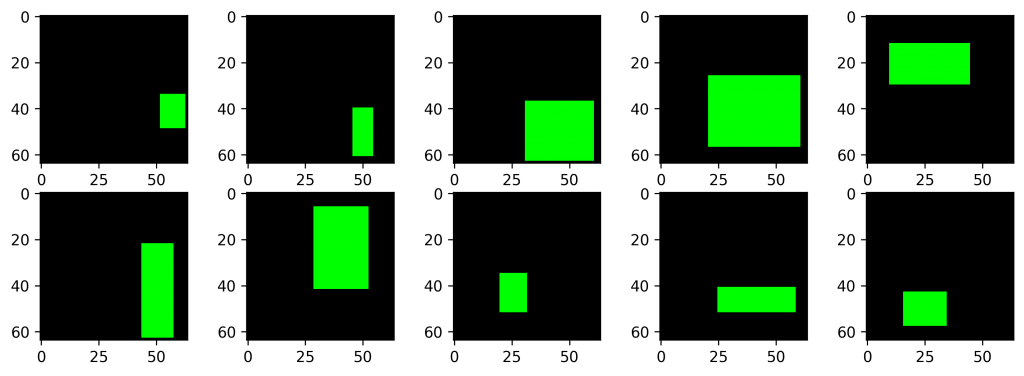

Prepare Data

First of all, I will normalize the input data to be centered around 0. The RGB values are within 0 and 255. Hence, I can just divide the feature tensor by 255, so that all values are within 0 to 1 and can then subtract 0.5, to center the values.

# normalize images
X = X.astype("float32") / 255
# center pixel values
X = X - 0.5

Furthermore, I split the data into a training, validation, and test set, using sklearn’s train_test_split function.

from sklearn.model_selection import train_test_split

X_train_val, X_test, Y_train_val, Y_test = train_test_split(X, Y, test_size=0.2)

# further split train_val
X_train, X_val, Y_train, Y_val = train_test_split(X_train_val, Y_train_val, test_size=0.2, random_state=29)

print("Shape X train:\t  ", X_train.shape)
print("Shape X validate: ", X_val.shape)
print("Shape X test:\t  ", X_test.shape)

# Output:
# Shape X train:       (25600, 64, 64, 3)
# Shape X validate:    (6400, 64, 64, 3)
# Shape X test:	       (8000, 64, 64, 3)

Convolutional Neural Network

Now it’s time to build the model. I use the Keras Sequential class as I will only use a linear stack of layers.

from tensorflow.keras.models import Sequential
from tensorflow.keras.layers import Conv2D, MaxPooling2D, Dense
from tensorflow.keras.layers import Flatten, Dropout

model = Sequential([
    Conv2D( 32, kernel_size=3, activation="relu",
           input_shape=(image_size, image_size, 3)),
    MaxPooling2D( pool_size=2),
    Conv2D( 32, kernel_size=3, activation="relu"),
    MaxPooling2D( pool_size=2),
    Flatten(),
    Dropout(0.5),
    Dense(4)
])

model.compile("adam", loss="mse", metrics=["accuracy"])

The model is kept simple, with two blocks consisting of a convolutional layer, followed by a max pooling layer. Finally, the input is flattened and connected to a dense layer with 4 nodes, which represents the target vector (x, y, w, h).

I use Adam as Optimizer and as loss the mean squared error, as the target is rather continuous.

Time to start the training!

%%time
epochs = 18
history = model.fit(X_train, Y_train,
                    epochs=epochs,
                    validation_data=(X_val, Y_val))

With my setup (GPU: Nvidia GeForce GTX 1050 Ti, CPU: Intel i5-3470) the training takes about 2 minutes and 26 seconds.

Results

When plotting the history of the training process I get the following results:

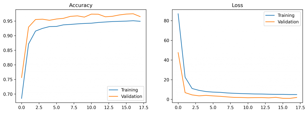
Let’s evaluate the model on (unseen) test data.

loss, acc = model.evaluate(X_test, Y_test)
print("Accuracy: %.4f"%acc)
print("Loss: %.4f"%loss)

# Output:
# Accuracy: 0.9729
# Loss: 1.6682

An accuracy of about 97% seems quite good. However, the accuracy may not be an appropriate indicator of how well the model performs in detecting objects. So we need to consider another measure, namely the Intersection over Union (IoU), which is more common to evaluate object detection accuracy.

What is IoU? In short, the Intersection over Union measures the overlap between two bounding boxes. A value of 1 indicates perfect prediction, while lower values suggest a poor accuracy.

Note: If you want to know more about the IoU, I would recommend to read this post.

So for the evaluation of the model, I will compute the IoU for all samples of the test set:

# predict test set
preds = model.predict(X_test)

# compute mean IoU
iou_all = []
for i in range(len(Y_test)):
    iou_arr.append(computeIoU(Y_test[i], preds[i]))
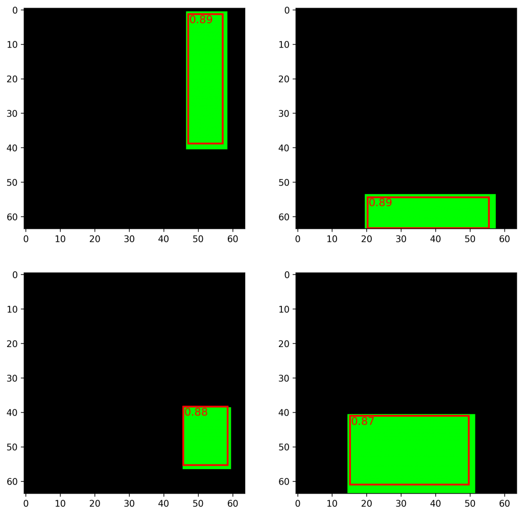
print("Mean IoU over Test Set: %.4f"%(np.mean(iou_all)))

Finally for the whole test set I get a mean IoU of 0.81. Not so bad for the first try. Below you can see the first four rectangles and their predicted bounding box, as well as the IoU.

Sample detection of the test data set, and the corresponding IoU.

Conclusion

We build a simple object localization model that is able to locate a rectangle on a neutral background. However, this model is not able to detect multiple objects, nor can it distinguish a rectangle from another shape, e.g. a circle. In the next post I would like to describe my second approach towards object detection, where I will tackle these problems.

If you have any comments or doubts about what I’ve done so far, feel free to leave a comment. 🙂

Github Repo: https://github.com/joh-fischer/object-localization